Blog

  • 2-bridge knot

    2-bridge knot
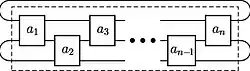
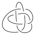
    Schematic picture of a 2-bridge knot.
    Bridge number 2
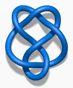
    2-bridge knot
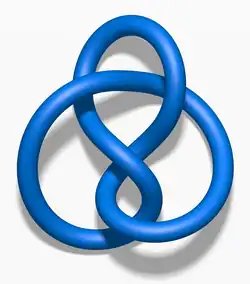
    31
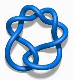
    2-bridge knot
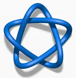
    51
    2-bridge knot
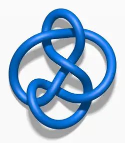
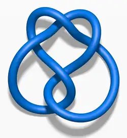
    63
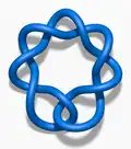
    2-bridge knot
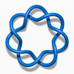
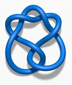
    71

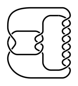
    In the mathematical field of knot theory, a 2-bridge knot is a knot which can be regular isotoped so that the natural height function given by the z-coordinate has only two maxima and two minima as critical points. Equivalently, these are the knots with bridge number 2, the smallest possible bridge number for a nontrivial knot. Every nontrivial knot with up to seven crossings is a 2-bridge knot. The simplest knots with a bridge number of 3 have eight crossings. Of the 1,701,936 knots with up to sixteen crossings, 5,546 are 2-bridge knots.[1]

    Other names for 2-bridge knots are rational knots, 4-plats, and Viergeflechte (German for four braids). 2-bridge links are defined similarly as above, but each component will have one min and max. 2-bridge knots were classified by Horst Schubert, using the fact that the 2-sheeted branched cover of the 3-sphere over the knot is a lens space.

    Schubert normal form

    The names rational knot and rational link were coined by John Conway who defined them as arising from numerator closures of rational tangles.
    This definition can be used to give a bijection between the set of 2-bridge links and the set of rational numbers; the rational number associated to a given link is called
    the Schubert normal form of the link (as this invariant was first defined by Schubert[2]), and is precisely the fraction associated to the rational tangle whose numerator closure gives the link.[3]:chapter 10

    Further reading

    • Louis H. Kauffman, Sofia Lambropoulou: On the classification of rational knots, L’ Enseignement Mathématique, 49:357410 (2003). preprint available at arxiv.org
    • C. C. Adams, The Knot Book: An elementary introduction to the mathematical theory of knots. American Mathematical Society, Providence, RI, 2004. xiv+307 pp. ISBN 0-8218-3678-1

    References

    1. De Wit, David (2007). “THE 2-BRIDGE KNOTS OF UP TO 16 CROSSINGS” (PDF). Journal of Knot Theory and Its Ramifications. 16 (08): 997–1019. doi:10.1142/S021821650700566X. ISSN 0218-2165. Retrieved 2025-09-06.
    2. Schubert, Horst (1956). “Knoten mit zwei Brücken”. Mathematische Zeitschrift. 65: 133–170. doi:10.1007/bf01473875.
    3. Purcell, Jessica (2020). Hyperbolic knot theory. American Mathematical Society. ISBN 978-1-4704-5499-9.

    External links


    This article is adapted from “2-bridge knot” on Wikipedia, written by its contributors, and used under CC BY-SA 4.0. Text on this page is available under the same licence. Source snapshot: Wikipedia via Kiwix, 2026-07-20.

  • Lucet

    Lucet
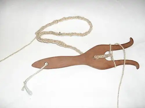
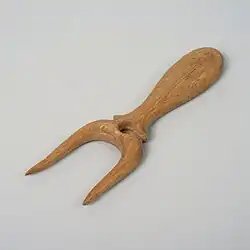
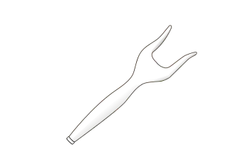
    Wooden, lyre-shaped lucet, with in-progress square cord

    A lucet is a tool used in cordmaking or braiding which is believed to date back to the Viking[1] and Medieval[2] periods, when it was used to create cords that were used on clothing,[1] or to hang items from the belt.[3] Lucet cord is square, strong, and slightly springy. It closely resembles knitted I-cord or the cord produced on a knitting spool. Lucet may unravel if cut, but is easily fixed with a small knot. Unlike other braiding techniques such as kumihimo, finger-loop braiding or plaiting, where the threads are of a finite length, lucetted (or knitted)[a] braids can be created without pre-measuring threads and so it is a technique suited for very long cords.

    Origins of the lucet

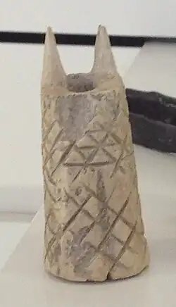
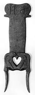
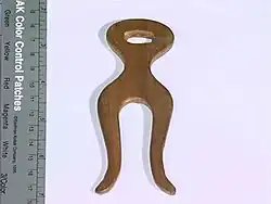
    The supposed medieval lucets appear to be double-pronged hollow bones, left tubular, presumably so that the cord could be drawn through the centre hole.[2] In contrast, a modern lucet fork is lyre-shaped, normally made of wood, with two prongs at one end and (optionally) a handle on the other. It may also have a hole through which the cord can be pulled.

    The exact origins of the lucet are controversial. While it was previously suggested that its use declined after the 12th century,[2] revived in the 17th century,[4] then waned again in the early 19th century;[3] the historical identification of lucets in archaeological digs is tricky. The biggest challenge in identifying ancient lucets is that their design is simple, making it difficult to distinguish from other two-pronged tools. Many presumed lucets were made from bones, branches, or antlers, and are often misidentified by archaeologists.[5]

    For example, a two-pronged 11th-century finding from Lund (Sweden)[6] has been associated with lucetting due to its design and runic inscription. This artifact, despite having features that suggest its use in cordmaking, is debated among experts. In York, both bone and antler finds have been catalogued as lucets,[7] although some, particularly the antler finds, are considered too impractical for weaving due to their divergent prongs and wear marks consistent with pendants.
    [8]

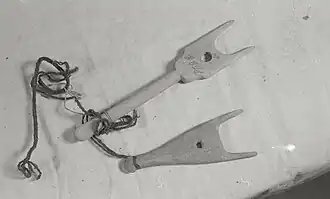
    The absence of a universally recognized shape for a lucet further complicates this identification. Findings range from hollow bones with two prongs, sometimes bearing a third larger prong, to small flat tools. Artifacts associated with medieval textile crafts, such as those found in Sigtuna (Sweden),[9] Wandignies-Hamage (France),[10] and other Northern European sites,[11] have been re-examined through experimental archaeology, supporting their potential use as lucets, although doubts persist. Despite this, the term ‘lucet’ has been applied to similar objects, especially those found in textile-related contexts.

    Construction of lucet braid

    • 10th-century lucet spool from northern France
      10th-century lucet spool from northern France
    • Lucet
    • Lucet

    A number of techniques exist for the creation of lucet cord, all of which produce slightly different cords; it is possible to produce a two-coloured cord by using two strands of differently-coloured yarn. The only materials necessary to lucet are yarn and a lucet fork, also known as a chain fork or a lucet. Skewer-like sticks or knitting needles can be used to pull the yarn over as an additional tool. Lucets can be bought in shops as kits designed for children.

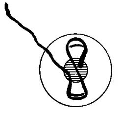
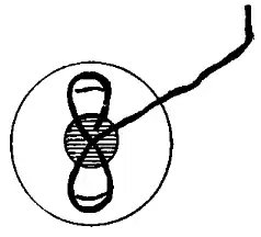
    To cast on, the yarn is put through the hole in the lucet from the front, and the yarn in front of the lucet is wound around the prongs twice, in a figure-of-eight motion. The two lower loops are then lifted over the two upper loops, using either the fingers or a stick, until they are lifted over the ‘horns’ of the lucet fork, after which the thread behind the lucet is pulled to tighten the knot. The process is then repeated, this time (and every time after) winding the yarn just once around the prongs, as there is already a figure-of-eight of yarn on the fork.

    When the desired length of lucet cord is reached, the lucet can be cast off by carefully lifting the loops off the prongs, passing the remaining thread through them, and pulling the knot tight. Any loose thread can be cut off with scissors, or tied together to form a closed circle. The cord can be wrapped around the lucet handle as it grows.

    Lucet cord can be used for decorative edging, draw-strings, lacing, and any other use where a strong cord is needed.

    • Lucet
    • Lucet
    • Lucet
    • Lucet
    • Lucet

    See also

    • Spool knitting, more general, with two or more horns.

    Notes

    1. The term lucet is used as a verb to describe the process of creating lucet cord, as in “to lucet”, “lucetted” and “lucetting”, as well as being a noun used to describe the resulting cord itself, and a noun used to describe the tool used in the cords’ creation.

    References

    1. 1 2 Pettersson, Kerstin (1968). “En gotländsk kvinnas dräkt. Kring ett textilfynd från vikingatiden”. TOR (in Swedish) (12). Uppsala: Societas Archaelogica Upsaliensis: 174–200.
    2. 1 2 3 MacGregor, Arthur (1985). Bone, Antler, Ivory and Horn: The Technology of Skeletal Materials since the Roman Period. London: Croom Helm.
    3. 1 2 Groves, Sylvia (1966). The History of Needlework Tools and Accessories. Middlesex: Hamlyn Publishing.
    4. Oxford English Dictionary. See: Lucet obs.
    5. Rossi, Sara; Phelps, Daniel (2023). “The Lucet Compendium: A Historical Exploration and Practical Guide”. The Compleat Anachronist (202). Milpitas, CA: Society for Creative Anachronism.
    6. Steenholt Olesen, Rikke (September 2021). “Et tinbl:Bein fra Middelalderens Lund: Et tekstilredskab – men hvilket?”. Danske Studier: 5–24. doi:10.7146/danskestudier.vi.128793.
    7. Walton Rogers, Penelope (1997). Textile Production at 16–22 Coppergate. York: Council for British Archaeology. p. 1790.
    8. Nutz, Beatrix (2024). Rieser, Anna (ed.). UFOs stricken – das Phantom der spätantiken/mittelalterlichen “Strickgabeln”. NEARCHOS. Vol. 25. Darmstadt: Verlag Marie Leidorf. pp. 245–262.
    9. Haltiner, S. (1990). Tesch, S. (ed.). Textilhantverk II – nålar och tinbl bein. Vol. Makt och människor i kungens Sigtuna. Sigtunautgrävningen 1988-90. Sigtuna: Sigtuna Museer.
    10. Étienne, Louis (2015). “Les indices d’artisanat dans et autour du monastère de Hamage (Nord)”. Bulletin du centre d’études médiévales d’Auxerre. Hors-série n° 8.
    11. Nutz, Beatrix (2022). Cords, Braids and Bands in Archaeology – Finds from Tyrol. Vol. Strands. pp. 3–9.

    This article is adapted from “Lucet” on Wikipedia, written by its contributors, and used under CC BY-SA 4.0. Text on this page is available under the same licence. Source snapshot: Wikipedia via Kiwix, 2026-07-20.

  • (−2,3,7) pretzel knot

    (−2,3,7) pretzel knot
    (−2,3,7) pretzel knot
    Arf invariant 0
    Crosscap no. 2
    Crossing no. 12
    Hyperbolic volume 2.828122
    Unknotting no. 5
    Conway notation [−2,3,7]
    Dowker notation 4, 8, -16, 2, -18, -20, -22, -24, -6, -10, -12, -14
    D–T notation 12n242
    Last / Next 12n241  / 12n243 
    Other
    hyperbolic, fibered, pretzel, reversible

    In geometric topology, a branch of mathematics, the (2, 3, 7) pretzel knot, sometimes called the Fintushel–Stern knot (after Ron Fintushel and Ronald J. Stern), is an important example of a pretzel knot which exhibits various interesting phenomena under three-dimensional and four-dimensional surgery constructions.

    Mathematical properties

    The (2, 3, 7) pretzel knot has 7 exceptional slopes, Dehn surgery slopes which give non-hyperbolic 3-manifolds. Among the enumerated knots, the only other hyperbolic knot with 7 or more is the figure-eight knot, which has 10. All other hyperbolic knots are conjectured to have at most 6 exceptional slopes.

    (−2,3,7) pretzel knot
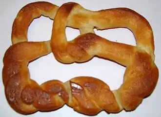
    A pretzel (−2,3,7) pretzel knot.

    Further reading

    • Kirby, R., (1978). “Problems in low dimensional topology”, Proceedings of Symposia in Pure Math., volume 32, 272–312. (see problem 1.77, due to Gordon, for exceptional slopes)

    External links


    This article is adapted from “(−2,3,7) pretzel knot” on Wikipedia, written by its contributors, and used under CC BY-SA 4.0. Text on this page is available under the same licence. Source snapshot: Wikipedia via Kiwix, 2026-07-20.

  • Loop representation in gauge theories and quantum gravity

    Beyond the Standard Model
    Loop representation in gauge theories and quantum gravity

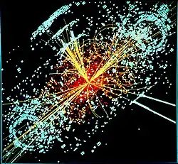
    Simulated Large Hadron Collider CMS particle detector data depicting a Higgs boson produced by colliding protons decaying into hadron jets and electrons
    Standard Model
    Evidence
    • Hierarchy problem
    • Dark matter
    • Dark energy
    • Quintessence
    • Phantom energy
    • Dark radiation
    • Dark photon
    • Cosmological constant problem
    • Strong CP problem
    • Neutrino oscillation
    Theories
    • Brans–Dicke theory
    • Cosmic censorship hypothesis
    • Fifth force
    • F-theory
    • Theory of everything
    • Unified field theory
    • Grand Unified Theory
    • Technicolor
    • Kaluza–Klein theory
    • 6D (2,0) superconformal field theory
    • Noncommutative quantum field theory
    • Quantum cosmology
    • Brane cosmology
    • String theory
    • Superstring theory
    • M-theory
    • Mathematical universe hypothesis
    • Mirror matter
    • Randall–Sundrum model
    • N = 4 supersymmetric Yang–Mills theory
    • Twistor string theory
    • Dark fluid
    • Doubly special relativity
    • de Sitter invariant special relativity
    • Causal fermion systems
    • Black hole thermodynamics
    • Unparticle physics
    • Graviphoton
    • Graviscalar
    • Graviton
    • Gravitino
    • Massive gravity
    • Gauge gravitation theory
    • Gauge theory gravity
    • CPT symmetry
    Supersymmetry
    • MSSM
    • NMSSM
    • Superstring theory
    • M-theory
    • Supergravity
    • Supersymmetry breaking
    • Extra dimensions
    • Large extra dimensions
    Quantum gravity
    • False vacuum
    • String theory
    • Spin foam
    • Quantum foam
    • Quantum geometry
    • Loop quantum gravity
    • Quantum cosmology
    • Loop quantum cosmology
    • Causal dynamical triangulation
    • Causal fermion systems
    • Causal sets
    • Canonical quantum gravity
    • Semiclassical gravity
    • Superfluid vacuum theory
    Experiments
    • ANNIE
    • Gran Sasso
    • INO
    • LHC
    • SNO
    • Super-K
    • Tevatron
    • NOvA

    Attempts have been made to describe gauge theories in terms of extended objects such as Wilson loops and holonomies. The loop representation is a quantum hamiltonian representation of gauge theories in terms of loops. The aim of the loop representation in the context of Yang–Mills theories is to avoid the redundancy introduced by Gauss gauge symmetries allowing to work directly in the space of physical states (Gauss gauge invariant states). The idea is well known in the context of lattice Yang–Mills theory (see lattice gauge theory). Attempts to explore the continuous loop representation was made by Gambini and Trias for canonical Yang–Mills theory, however there were difficulties as they represented singular objects. As we shall see the loop formalism goes far beyond a simple gauge invariant description, in fact it is the natural geometrical framework to treat gauge theories and quantum gravity in terms of their fundamental physical excitations.

    The introduction by Ashtekar of a new set of variables (Ashtekar variables) cast general relativity in the same language as gauge theories and allowed one to apply loop techniques as a natural nonperturbative description of Einstein’s theory. In canonical quantum gravity the difficulties in using the continuous loop representation are cured by the spatial diffeomorphism invariance of general relativity. The loop representation also provides a natural solution of the spatial diffeomorphism constraint, making a connection between canonical quantum gravity and knot theory. Surprisingly there were a class of loop states that provided exact (if only formal) solutions to Ashtekar’s original (ill-defined) Wheeler–DeWitt equation.[1] Hence an infinite set of exact (if only formal) solutions had been identified for all the equations of canonical quantum general gravity in this representation! This generated a lot of interest in the approach and eventually led to loop quantum gravity (LQG).

    The loop representation has found application in mathematics. If topological quantum field theories are formulated in terms of loops, the resulting quantities should be what are known as knot invariants. Topological field theories only involve a finite number of degrees of freedom and so are exactly solvable. As a result, they provide concrete computable expressions that are invariants of knots. This was precisely the insight of Edward Witten[2] who noticed that computing loop dependent quantities in Chern–Simons and other three-dimensional topological quantum field theories one could come up with explicit, analytic expressions for knot invariants. For his work in this, in 1990 he was awarded the Fields Medal. He is the first and so far the only physicist to be awarded the Fields Medal, often viewed as the greatest honour in mathematics.

    Gauge invariance of Maxwell’s theory

    The idea of gauge symmetries was introduced in Maxwell’s theory. Maxwell’s equations are

    E = ρ ϵ 0 × B ϵ 0 μ 0 E t = μ 0 J × E + B t = 0 B = 0 {\displaystyle \nabla \cdot {\vec {E}}={\rho \over \epsilon _{0}}\qquad \nabla \times {\vec {B}}-\epsilon _{0}\mu _{0}{\partial {\vec {E}} \over \partial t}=\mu _{0}{\vec {J}}\qquad \nabla \times {\vec {E}}+{\partial {\vec {B}} \over \partial t}=0\qquad \nabla \cdot {\vec {B}}=0} {\displaystyle \nabla \cdot {\vec {E}}={\rho  \over \epsilon _{0}}\qquad \nabla \times {\vec {B}}-\epsilon _{0}\mu _{0}{\partial {\vec {E}} \over \partial t}=\mu _{0}{\vec {J}}\qquad \nabla \times {\vec {E}}+{\partial {\vec {B}} \over \partial t}=0\qquad \nabla \cdot {\vec {B}}=0}

    where ρ {\displaystyle \rho } {\displaystyle \rho } is the charge density and J {\displaystyle {\vec {J}}} {\displaystyle {\vec {J}}} the current density. The last two equations can be solved by writing fields in terms of a scalar potential, ϕ {\displaystyle \phi } {\displaystyle \phi }, and a vector potential, A {\displaystyle {\vec {A}}} {\displaystyle {\vec {A}}}:

    E = ϕ A t B = × A {\displaystyle {\vec {E}}=-\nabla \phi -{\partial {\vec {A}} \over \partial t}\qquad {\vec {B}}=\nabla \times {\vec {A}}} {\displaystyle {\vec {E}}=-\nabla \phi -{\partial {\vec {A}} \over \partial t}\qquad {\vec {B}}=\nabla \times {\vec {A}}}.

    The potentials uniquely determine the fields, but the fields do not uniquely determine the potentials – we can make the changes:

    ϕ = ϕ + Λ t A = A Λ {\displaystyle \phi ‘=\phi +{\partial \Lambda \over \partial t}\qquad {\vec {A}}’={\vec {A}}-\nabla \Lambda } {\displaystyle \phi '=\phi +{\partial \Lambda  \over \partial t}\qquad {\vec {A}}'={\vec {A}}-\nabla \Lambda }

    without affecting the electric and magnetic fields, where Λ ( x , t ) {\displaystyle \Lambda ({\vec {x}},t)} {\displaystyle \Lambda ({\vec {x}},t)} is an arbitrary function of space-time . These are called gauge transformations. There is an elegant relativistic notation: the gauge field is

    A μ = ( ϕ , A ) {\displaystyle A^{\mu }=(\phi ,{\vec {A}})} {\displaystyle A^{\mu }=(\phi ,{\vec {A}})}

    and the above gauge transformations read,

    A μ = A μ + μ Λ {\displaystyle {A^{\mu }}’=A^{\mu }+\partial ^{\mu }\Lambda } {\displaystyle {A^{\mu }}'=A^{\mu }+\partial ^{\mu }\Lambda }.

    The so-called field strength tensor is introduced,

    F μ ν = μ A ν ν A μ {\displaystyle F^{\mu \nu }=\partial ^{\mu }A^{\nu }-\partial ^{\nu }A^{\mu }} {\displaystyle F^{\mu \nu }=\partial ^{\mu }A^{\nu }-\partial ^{\nu }A^{\mu }}

    which is easily shown to be invariant under gauge transformations. In components,

    F 0 i = E i , ϵ i j k F j k = B i {\displaystyle F^{0i}=E^{i},\qquad \epsilon ^{ijk}F^{jk}=B^{i}} {\displaystyle F^{0i}=E^{i},\qquad \epsilon ^{ijk}F^{jk}=B^{i}}.

    Maxwell’s source-free action is given by:

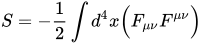
    S = 1 2 d 4 x ( F μ ν F μ ν ) {\displaystyle S=-{1 \over 2}\int d^{4}x{\Big (}F_{\mu \nu }F^{\mu \nu }{\Big )}} {\displaystyle S=-{1 \over 2}\int d^{4}x{\Big (}F_{\mu \nu }F^{\mu \nu }{\Big )}}.

    The ability to vary the gauge potential at different points in space and time (by changing Λ ( x , t ) {\displaystyle \Lambda ({\vec {x}},t)} {\displaystyle \Lambda ({\vec {x}},t)}) without changing the physics is called a local invariance. Electromagnetic theory possess the simplest kind of local gauge symmetry called U ( 1 ) {\displaystyle U(1)} {\displaystyle U(1)} (see unitary group). A theory that displays local gauge invariance is called a gauge theory. In order to formulate other gauge theories we turn the above reasoning inside out. This is the subject of the next section.

    The connection and gauges theories

    The connection and Maxwell’s theory

    We know from quantum mechanics that if we replace the wave-function, ψ ( x ) {\displaystyle \psi (x)} {\displaystyle \psi (x)}, describing the electron field by

    ψ ( x ) = exp ( i θ ) ψ ( x ) {\displaystyle \psi ‘(x)=\exp(i\theta )\psi (x)} {\displaystyle \psi '(x)=\exp(i\theta )\psi (x)}

    that it leaves physical predictions unchanged. We consider the imposition of local invariance on the phase of the electron field,

    ψ ( x ) = Ω ψ ( x ) = exp ( i θ ( x ) ) ψ ( x ) {\displaystyle \psi ‘(x)=\Omega \psi (x)=\exp(i\theta (x))\psi (x)} {\displaystyle \psi '(x)=\Omega \psi (x)=\exp(i\theta (x))\psi (x)}

    The problem is that derivatives of ψ ( x ) {\displaystyle \psi (x)} {\displaystyle \psi (x)} are not covariant under this transformation:

    μ ( exp ( i θ ( x ) ) ψ ( x ) ) = Ω μ ψ ( x ) + μ Ω ψ ( x ) {\displaystyle \partial _{\mu }(\exp(i\theta (x))\psi (x))=\Omega \partial _{\mu }\psi (x)+\partial _{\mu }\Omega \psi (x)} {\displaystyle \partial _{\mu }(\exp(i\theta (x))\psi (x))=\Omega \partial _{\mu }\psi (x)+\partial _{\mu }\Omega \psi (x)}.

    In order to cancel out the second unwanted term, one introduces a new derivative operator D μ {\displaystyle {\mathcal {D}}_{\mu }} {\displaystyle {\mathcal {D}}_{\mu }} that is covariant. To construct D μ {\displaystyle {\mathcal {D}}_{\mu }} {\displaystyle {\mathcal {D}}_{\mu }}, one introduces a new field, the connection A μ {\displaystyle A_{\mu }} {\displaystyle A_{\mu }}:

    D μ = μ + i g A μ ( x ) {\displaystyle {\mathcal {D}}_{\mu }=\partial _{\mu }+igA_{\mu }(x)} {\displaystyle {\mathcal {D}}_{\mu }=\partial _{\mu }+igA_{\mu }(x)}.

    Then

    ( D μ ψ ) = μ ψ + i g A μ ψ = Ω μ ψ + ( Ω ) ψ + i g A μ Ω ψ {\displaystyle ({\mathcal {D}}_{\mu }\psi )’=\partial _{\mu }\psi ‘+igA_{\mu }’\psi ‘=\Omega \partial _{\mu }\psi +(\partial \Omega )\psi +igA_{\mu }’\Omega \psi } {\displaystyle ({\mathcal {D}}_{\mu }\psi )'=\partial _{\mu }\psi '+igA_{\mu }'\psi '=\Omega \partial _{\mu }\psi +(\partial \Omega )\psi +igA_{\mu }'\Omega \psi }

    The term μ Ω {\displaystyle \partial _{\mu }\Omega } {\displaystyle \partial _{\mu }\Omega } is precisely cancelled out by requiring the connection field transforms as

    A μ ( x ) = A μ ( x ) + i g [ μ Ω ( x ) ] Ω 1 ( x ) E q 1. {\displaystyle A_{\mu }'(x)=A_{\mu }(x)+{i \over g}[\partial _{\mu }\Omega (x)]\Omega ^{-1}(x)\quad Eq1.} {\displaystyle A_{\mu }'(x)=A_{\mu }(x)+{i \over g}[\partial _{\mu }\Omega (x)]\Omega ^{-1}(x)\quad Eq1.}.

    We then have that

    ( D μ ψ ) = Ω D μ ψ {\displaystyle ({\mathcal {D}}_{\mu }\psi )’=\Omega {\mathcal {D}}_{\mu }\psi } {\displaystyle ({\mathcal {D}}_{\mu }\psi )'=\Omega {\mathcal {D}}_{\mu }\psi }.

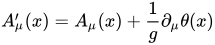
    Note that E q 1 {\displaystyle Eq1} {\displaystyle Eq1} is equivalent to

    A μ ( x ) = A μ ( x ) + 1 g μ θ ( x ) {\displaystyle A_{\mu }'(x)=A_{\mu }(x)+{1 \over g}\partial _{\mu }\theta (x)} {\displaystyle A_{\mu }'(x)=A_{\mu }(x)+{1 \over g}\partial _{\mu }\theta (x)}

    which looks the same as a gauge transformation of the gauge potential of Maxwell’s theory. It is possible to construct an invariant action for the connection field itself. We want an action that only has two derivatives (since actions with higher derivatives are not unitary). Define the quantity:

    F μ ν = i g [ D μ , D μ ] = i g [ μ + i g A μ ( x ) , ν + i g A ν ( x ) ] {\displaystyle F_{\mu \nu }={-i \over g}[{\mathcal {D}}_{\mu },{\mathcal {D}}_{\mu }]={-i \over g}[\partial _{\mu }+igA_{\mu }(x),\partial _{\nu }+igA_{\nu }(x)]} {\displaystyle F_{\mu \nu }={-i \over g}[{\mathcal {D}}_{\mu },{\mathcal {D}}_{\mu }]={-i \over g}[\partial _{\mu }+igA_{\mu }(x),\partial _{\nu }+igA_{\nu }(x)]}

    = i g ( [ μ , ν ] + i g ( μ A ν ν A μ ) g 2 [ A μ , A ν ] ) {\displaystyle ={-i \over g}{\Big (}[\partial _{\mu },\partial _{\nu }]+ig(\partial _{\mu }A_{\nu }-\partial _{\nu }A_{\mu })-g^{2}[A_{\mu },A_{\nu }]{\Big )}} {\displaystyle ={-i \over g}{\Big (}[\partial _{\mu },\partial _{\nu }]+ig(\partial _{\mu }A_{\nu }-\partial _{\nu }A_{\mu })-g^{2}[A_{\mu },A_{\nu }]{\Big )}}

    = μ A ν ν A ν {\displaystyle =\partial _{\mu }A_{\nu }-\partial _{\nu }A_{\nu }} {\displaystyle =\partial _{\mu }A_{\nu }-\partial _{\nu }A_{\nu }}.

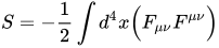
    The unique action with only two derivatives is given by:

    S = 1 2 d 4 x ( F μ ν F μ ν ) {\displaystyle S=-{\frac {1}{2}}\int d^{4}x{\Big (}F_{\mu \nu }F^{\mu \nu }{\Big )}} {\displaystyle S=-{\frac {1}{2}}\int d^{4}x{\Big (}F_{\mu \nu }F^{\mu \nu }{\Big )}}.

    Therefore, one can derive electromagnetic theory from arguments based solely on symmetry.

    The connection and Yang-Mills gauge theory

    We now generalize the above reasoning to general gauge groups. One begins with the generators of some Lie algebra:

    [ T i , T j ] = i f i j k T k {\displaystyle [T_{i},T_{j}]=if^{ijk}T^{k}} {\displaystyle [T_{i},T_{j}]=if^{ijk}T^{k}}

    Let there be a fermion field that transforms as

    Ψ Ω ^ ( x ) Ψ ( x ) = exp ( i θ i ( x ) T i ) Ψ ( x ) {\displaystyle \mathbf {\Psi } ‘\mapsto {\hat {\Omega }}(x)\mathbf {\Psi } (x)=\exp(i\theta ^{i}(x)T^{i})\mathbf {\Psi } (x)} {\displaystyle \mathbf {\Psi } '\mapsto {\hat {\Omega }}(x)\mathbf {\Psi } (x)=\exp(i\theta ^{i}(x)T^{i})\mathbf {\Psi } (x)}

    Again the derivatives of Ψ ( x ) {\displaystyle \mathbf {\Psi } (x)} {\displaystyle \mathbf {\Psi } (x)} are not covariant under this transformation. We introduce a covariant derivative

    D μ = I μ + i g A μ ( x ) {\displaystyle \mathbf {\mathcal {D}} _{\mu }=\mathbf {I} \partial _{\mu }+ig\mathbf {A} _{\mu }(x)} {\displaystyle \mathbf {\mathcal {D}} _{\mu }=\mathbf {I} \partial _{\mu }+ig\mathbf {A} _{\mu }(x)}

    with connection field given by

    A μ ( x ) = A μ i ( x ) T i {\displaystyle \mathbf {A} _{\mu }(x)=A_{\mu }^{i}(x)T^{i}} {\displaystyle \mathbf {A} _{\mu }(x)=A_{\mu }^{i}(x)T^{i}}

    We require that A μ ( x ) {\displaystyle \mathbf {A} _{\mu }(x)} {\displaystyle \mathbf {A} _{\mu }(x)} transforms as:

    A μ ( x ) = Ω ^ A μ ( x ) Ω ^ 1 + i g Ω ^ ( μ Ω ^ 1 ) {\displaystyle \mathbf {A} _{\mu }'(x)={\hat {\Omega }}\mathbf {A} _{\mu }(x){\hat {\Omega }}^{-1}+{i \over g}{\hat {\Omega }}(\partial _{\mu }{\hat {\Omega }}^{-1})} {\displaystyle \mathbf {A} _{\mu }'(x)={\hat {\Omega }}\mathbf {A} _{\mu }(x){\hat {\Omega }}^{-1}+{i \over g}{\hat {\Omega }}(\partial _{\mu }{\hat {\Omega }}^{-1})}.

    We define the field strength operator

    F μ ν = i g [ D μ , D ν ] = μ A ν ν A μ + i g [ A μ , A ν ] = ( μ A ν i ν A μ i + g f i j k A μ j A ν k ) T i {\displaystyle \mathbf {F} _{\mu \nu }=-{i \over g}[\mathbf {\mathcal {D}} _{\mu },\mathbf {\mathcal {D}} _{\nu }]=\partial _{\mu }\mathbf {A} _{\nu }-\partial _{\nu }\mathbf {A} _{\mu }+ig[\mathbf {A} _{\mu },\mathbf {A} _{\nu }]=(\partial _{\mu }A_{\nu }^{i}-\partial _{\nu }A_{\mu }^{i}+gf^{ijk}A_{\mu }^{j}A_{\nu }^{k})T^{i}} {\displaystyle \mathbf {F} _{\mu \nu }=-{i \over g}[\mathbf {\mathcal {D}} _{\mu },\mathbf {\mathcal {D}} _{\nu }]=\partial _{\mu }\mathbf {A} _{\nu }-\partial _{\nu }\mathbf {A} _{\mu }+ig[\mathbf {A} _{\mu },\mathbf {A} _{\nu }]=(\partial _{\mu }A_{\nu }^{i}-\partial _{\nu }A_{\mu }^{i}+gf^{ijk}A_{\mu }^{j}A_{\nu }^{k})T^{i}}.

    As D μ {\displaystyle \mathbf {\mathcal {D}} _{\mu }} {\displaystyle \mathbf {\mathcal {D}} _{\mu }} is covariant, this means that the F μ ν i {\displaystyle F_{\mu \nu }^{i}} {\displaystyle F_{\mu \nu }^{i}} tensor is also covariant:

    F μ ν F μ ν = Ω ^ F μ ν Ω ^ 1 {\displaystyle \mathbf {F} _{\mu \nu }\mapsto \mathbf {F} _{\mu \nu }’={\hat {\Omega }}\mathbf {F} _{\mu \nu }{\hat {\Omega }}^{-1}} {\displaystyle \mathbf {F} _{\mu \nu }\mapsto \mathbf {F} _{\mu \nu }'={\hat {\Omega }}\mathbf {F} _{\mu \nu }{\hat {\Omega }}^{-1}}

    Note that F μ ν {\displaystyle \mathbf {F} _{\mu \nu }} {\displaystyle \mathbf {F} _{\mu \nu }} is only invariant under gauge transformations if Ω ^ {\displaystyle {\hat {\Omega }}} {\displaystyle {\hat {\Omega }}} is a scalar, that is, only in the case of electromagnetism.

    We can now construct an invariant action out of this tensor. Again we want an action that only has two derivatives. The simplest choice is the trace of the commutator:

    Tr ( Ω ^ F μ ν Ω ^ 1 Ω ^ F μ ν Ω ^ 1 ) = Tr ( F μ ν F μ ν ) {\displaystyle \operatorname {Tr} ({\hat {\Omega }}\mathbf {F} _{\mu \nu }{\hat {\Omega }}^{-1}{\hat {\Omega }}\mathbf {F} ^{\mu \nu }{\hat {\Omega }}^{-1})=\operatorname {Tr} (\mathbf {F} _{\mu \nu }\mathbf {F} ^{\mu \nu })} {\displaystyle \operatorname {Tr} ({\hat {\Omega }}\mathbf {F} _{\mu \nu }{\hat {\Omega }}^{-1}{\hat {\Omega }}\mathbf {F} ^{\mu \nu }{\hat {\Omega }}^{-1})=\operatorname {Tr} (\mathbf {F} _{\mu \nu }\mathbf {F} ^{\mu \nu })}

    The unique action with only two derivatives is given by:

    S = 1 2 d 4 x T r ( F μ ν F μ ν ) = 1 2 d 4 x Tr ( F μ ν i T j F j μ ν T j ) {\displaystyle S=-{1 \over 2}\int d^{4}xTr(\mathbf {F} _{\mu \nu }\mathbf {F} ^{\mu \nu })=-{1 \over 2}\int d^{4}x\operatorname {Tr} {\Big (}F_{\mu \nu }^{i}T^{j}F_{j}^{\mu \nu }T^{j}{\Big )}} {\displaystyle S=-{1 \over 2}\int d^{4}xTr(\mathbf {F} _{\mu \nu }\mathbf {F} ^{\mu \nu })=-{1 \over 2}\int d^{4}x\operatorname {Tr} {\Big (}F_{\mu \nu }^{i}T^{j}F_{j}^{\mu \nu }T^{j}{\Big )}}

    This is the action for Yang-mills theory.

    The loop representation of the Maxwell theory

    We consider a change of representation in the quantum Maxwell gauge theory. The idea is to introduce a basis of states labeled by loops γ {\displaystyle \mid \gamma \rangle } {\displaystyle \mid \gamma \rangle } whose inner product with the connection states is given by

    A γ = W ( γ ) = exp [ i e γ d y α A α ( y ) ] {\displaystyle \langle A\mid \gamma \rangle =W(\gamma )=\exp \left[ie\int _{\gamma }dy^{\alpha }A_{\alpha }(y)\right]} {\displaystyle \langle A\mid \gamma \rangle =W(\gamma )=\exp \left[ie\int _{\gamma }dy^{\alpha }A_{\alpha }(y)\right]}

    The loop functional W ( γ ) {\displaystyle W(\gamma )} {\displaystyle W(\gamma )} is the Wilson loop for the abelian U ( 1 ) {\displaystyle U(1)} {\displaystyle U(1)} case.

    The loop representation of Yang–Mills theory

    We consider for simplicity (and because later we will see this is the relevant gauge group in LQG) an S U ( 2 ) {\displaystyle SU(2)} {\displaystyle SU(2)} Yang–Mills theory in four dimensions. The field variable of the continuous theory is an S U ( 2 ) {\displaystyle SU(2)} {\displaystyle SU(2)} connection (or gauge potential) A μ i ( x ) {\displaystyle A_{\mu }^{i}(x)} {\displaystyle A_{\mu }^{i}(x)}, where i {\displaystyle i} {\displaystyle i} is an index in the Lie algebra of S U ( 2 ) {\displaystyle SU(2)} {\displaystyle SU(2)}. We can write for this field

    A μ ( x ) = A μ i ( x ) τ i {\displaystyle \mathbf {A} _{\mu }(x)=A_{\mu }^{i}(x)\tau _{i}} {\displaystyle \mathbf {A} _{\mu }(x)=A_{\mu }^{i}(x)\tau _{i}}

    where τ i {\displaystyle \tau _{i}} {\displaystyle \tau _{i}} are the s u ( 2 ) {\displaystyle su(2)} {\displaystyle su(2)} generators, that is the Pauli matrices multiplied by i / 2 {\displaystyle i/2} {\displaystyle i/2}. note that unlike with Maxwell’s theory, the connections A μ ( x ) {\displaystyle \mathbf {A} _{\mu }(x)} {\displaystyle \mathbf {A} _{\mu }(x)} are matrix-valued and don’t commute, that is they are non-Abelian gauge theories. We must take this into account when defining the corresponding version of the holonomy for S U ( 2 ) {\displaystyle SU(2)} {\displaystyle SU(2)} Yang–Mills theory.

    We first describe the quantum theory in terms of connection variable.

    The connection representation

    In the connection representation the configuration variable is A a i {\displaystyle A_{a}^{i}} {\displaystyle A_{a}^{i}} and its conjugate momentum is the (densitized) triad E ~ i a {\displaystyle {\tilde {E}}_{i}^{a}} {\displaystyle {\tilde {E}}_{i}^{a}}. It is most natural to consider wavefunctions Ψ ( A a i ) {\displaystyle \Psi (A_{a}^{i})} {\displaystyle \Psi (A_{a}^{i})}. This is known as the connection representation. The canonical variables get promoted to quantum operators:

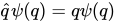
    A ^ a i Ψ [ A ] = A a i Ψ [ A ] {\displaystyle {\hat {A}}_{a}^{i}\Psi [A]=A_{a}^{i}\Psi [A]} {\displaystyle {\hat {A}}_{a}^{i}\Psi [A]=A_{a}^{i}\Psi [A]}

    (analogous to the position representation q ^ ψ ( q ) = q ψ ( q ) {\displaystyle {\hat {q}}\psi (q)=q\psi (q)} {\displaystyle {\hat {q}}\psi (q)=q\psi (q)}) and the triads are functional derivatives,

    E ~ ^ a i Ψ [ A ] = i δ Ψ [ A ] δ A a i {\displaystyle {\hat {\tilde {E}}}_{a}^{i}\Psi [A]=-i{\delta \Psi [A] \over \delta A_{a}^{i}}} {\displaystyle {\hat {\tilde {E}}}_{a}^{i}\Psi [A]=-i{\delta \Psi [A] \over \delta A_{a}^{i}}}

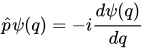
    (analogous to p ^ ψ ( q ) = i d ψ ( q ) d q {\displaystyle {\hat {p}}\psi (q)=-i{d\psi (q) \over dq}} {\displaystyle {\hat {p}}\psi (q)=-i{d\psi (q) \over dq}})

    The holonomy and Wilson loop

    Let us return to the classical Yang–Mills theory. It is possible to encode the gauge invariant information of the theory in terms of `loop-like’ variables.

    We need the notion of a holonomy. A holonomy is a measure of how much the initial and final values of a spinor or vector differ after parallel transport around a closed loop γ {\displaystyle \gamma } {\displaystyle \gamma }  ; it is denoted

    h γ [ A ] {\displaystyle h_{\gamma }[A]} {\displaystyle h_{\gamma }[A]}

    Knowledge of the holonomies is equivalent to knowledge of the connection, up to gauge equivalence. Holonomies can also be associated with an edge; under a Gauss Law these transform as

    ( h e ) α β = U α γ 1 ( x ) ( h e ) γ σ U σ β ( y ) . {\displaystyle (h’_{e})_{\alpha \beta }=U_{\alpha \gamma }^{-1}(x)(h_{e})_{\gamma \sigma }U_{\sigma \beta }(y).} {\displaystyle (h'_{e})_{\alpha \beta }=U_{\alpha \gamma }^{-1}(x)(h_{e})_{\gamma \sigma }U_{\sigma \beta }(y).}

    For a closed loop x = y {\displaystyle x=y} {\displaystyle x=y} if we take the trace of this, that is, putting α = β {\displaystyle \alpha =\beta } {\displaystyle \alpha =\beta } and summing we obtain

    ( h e ) α α = U α γ 1 ( x ) ( h e ) γ σ U σ α ( x ) = [ U σ α ( x ) U α γ 1 ( x ) ] ( h e ) γ σ = δ σ γ ( h e ) γ σ = ( h e ) γ γ {\displaystyle (h’_{e})_{\alpha \alpha }=U_{\alpha \gamma }^{-1}(x)(h_{e})_{\gamma \sigma }U_{\sigma \alpha }(x)=[U_{\sigma \alpha }(x)U_{\alpha \gamma }^{-1}(x)](h_{e})_{\gamma \sigma }=\delta _{\sigma \gamma }(h_{e})_{\gamma \sigma }=(h_{e})_{\gamma \gamma }} {\displaystyle (h'_{e})_{\alpha \alpha }=U_{\alpha \gamma }^{-1}(x)(h_{e})_{\gamma \sigma }U_{\sigma \alpha }(x)=[U_{\sigma \alpha }(x)U_{\alpha \gamma }^{-1}(x)](h_{e})_{\gamma \sigma }=\delta _{\sigma \gamma }(h_{e})_{\gamma \sigma }=(h_{e})_{\gamma \gamma }}

    or

    Tr h γ = Tr h γ . {\displaystyle \operatorname {Tr} h’_{\gamma }=\operatorname {Tr} h_{\gamma }.} {\displaystyle \operatorname {Tr} h'_{\gamma }=\operatorname {Tr} h_{\gamma }.}

    Thus the trace of an holonomy around a closed loop is gauge invariant. It is denoted

    W γ [ A ] {\displaystyle W_{\gamma }[A]} {\displaystyle W_{\gamma }[A]}

    and is called a Wilson loop. The explicit form of the holonomy is

    h γ [ A ] = P exp { γ 0 γ 1 d s γ ˙ a A a i ( γ ( s ) ) T i } {\displaystyle h_{\gamma }[A]={\mathcal {P}}\exp {\Big \{}-\int _{\gamma _{0}}^{\gamma _{1}}\,ds{\dot {\gamma }}^{a}A_{a}^{i}(\gamma (s))T_{i}{\Big \}}} {\displaystyle h_{\gamma }[A]={\mathcal {P}}\exp {\Big \{}-\int _{\gamma _{0}}^{\gamma _{1}}\,ds{\dot {\gamma }}^{a}A_{a}^{i}(\gamma (s))T_{i}{\Big \}}}

    where γ {\displaystyle \gamma } {\displaystyle \gamma } is the curve along which the holonomy is evaluated, and s {\displaystyle s} {\displaystyle s} is a parameter along the curve, P {\displaystyle {\mathcal {P}}} {\displaystyle {\mathcal {P}}} denotes path ordering meaning factors for smaller values of s {\displaystyle s} {\displaystyle s} appear to the left, and T i {\displaystyle T_{i}} {\displaystyle T_{i}} are matrices that satisfy the s u ( 2 ) {\displaystyle su(2)} {\displaystyle su(2)} algebra

    [ T i , T j ] = 2 i ϵ i j k T k . {\displaystyle [T^{i},T^{j}]=2i\epsilon ^{ijk}T^{k}.\,} {\displaystyle [T^{i},T^{j}]=2i\epsilon ^{ijk}T^{k}.\,}

    The Pauli matrices satisfy the above relation. It turns out that there are infinitely many more examples of sets of matrices that satisfy these relations, where each set comprises ( N + 1 ) × ( N + 1 ) {\displaystyle (N+1)\times (N+1)} {\displaystyle (N+1)\times (N+1)} matrices with N = 1 , 2 , 3 , {\displaystyle N=1,2,3,\dots } {\displaystyle N=1,2,3,\dots }, and where none of these can be thought to `decompose’ into two or more examples of lower dimension. They are called different irreducible representations of the s u ( 2 ) {\displaystyle su(2)} {\displaystyle su(2)} algebra. The most fundamental representation being the Pauli matrices. The holonomy is labelled by a half integer N / 2 {\displaystyle N/2} {\displaystyle N/2} according to the irreducible representation used.

    Giles’ Reconstruction theorem of gauge potentials from Wilson loops

    An important theorem about Yang–Mills gauge theories is Giles’ theorem, according to which if one gives the trace of the holonomy of a connection for all possible loops on a manifold one can, in principle, reconstruct all the gauge invariant information of the connection.[3] That is, Wilson loops constitute a basis of gauge invariant functions of the connection. This key result is the basis for the loop representation for gauge theories and gravity.

    The loop transform and the loop representation

    The use of Wilson loops explicitly solves the Gauss gauge constraint. As Wilson loops form a basis we can formally expand any Gauss gauge invariant function as,

    Ψ [ A ] = γ Ψ [ γ ] W γ [ A ] {\displaystyle \Psi [A]=\sum _{\gamma }\Psi [\gamma ]W_{\gamma }[A]} {\displaystyle \Psi [A]=\sum _{\gamma }\Psi [\gamma ]W_{\gamma }[A]}.

    This is called the loop transform. We can see the analogy with going to the momentum representation in quantum mechanics. There one has a basis of states exp ( i k x ) {\displaystyle \exp(ikx)} {\displaystyle \exp(ikx)} labelled by a number k {\displaystyle k} {\displaystyle k} and one expands

    ψ [ x ] = d k ψ ( k ) exp ( i k x ) . {\displaystyle \psi [x]=\int dk\psi (k)\exp(ikx).} {\displaystyle \psi [x]=\int dk\psi (k)\exp(ikx).}

    and works with the coefficients of the expansion ψ ( k ) {\displaystyle \psi (k)} {\displaystyle \psi (k)}.

    The inverse loop transform is defined by

    Ψ [ γ ] = [ d A ] Ψ [ A ] W γ [ A ] . {\displaystyle \Psi [\gamma ]=\int [dA]\Psi [A]W_{\gamma }[A].} {\displaystyle \Psi [\gamma ]=\int [dA]\Psi [A]W_{\gamma }[A].}

    This defines the loop representation. Given an operator O ^ {\displaystyle {\hat {O}}} {\displaystyle {\hat {O}}} in the connection representation,

    Φ [ A ] = O ^ Ψ [ A ] , Eq 1 {\displaystyle \Phi [A]={\hat {O}}\Psi [A],\qquad {\text{Eq 1}}} {\displaystyle \Phi [A]={\hat {O}}\Psi [A],\qquad {\text{Eq 1}}}

    one should define the corresponding operator O ^ {\displaystyle {\hat {O}}’} {\displaystyle {\hat {O}}'} on Ψ [ γ ] {\displaystyle \Psi [\gamma ]} {\displaystyle \Psi [\gamma ]} in the loop representation via,

    Φ [ γ ] = O ^ Ψ [ γ ] , Eq 2 {\displaystyle \Phi [\gamma ]={\hat {O}}’\Psi [\gamma ],\qquad {\text{Eq 2}}} {\displaystyle \Phi [\gamma ]={\hat {O}}'\Psi [\gamma ],\qquad {\text{Eq 2}}}

    where Φ [ γ ] {\displaystyle \Phi [\gamma ]} {\displaystyle \Phi [\gamma ]} is defined by the usual inverse loop transform,

    Φ [ γ ] = [ d A ] Φ [ A ] W γ [ A ] . Eq 3 {\displaystyle \Phi [\gamma ]=\int [dA]\Phi [A]W_{\gamma }[A].\qquad {\text{Eq 3}}} {\displaystyle \Phi [\gamma ]=\int [dA]\Phi [A]W_{\gamma }[A].\qquad {\text{Eq 3}}}

    A transformation formula giving the action of the operator O ^ {\displaystyle {\hat {O}}’} {\displaystyle {\hat {O}}'} on Ψ [ γ ] {\displaystyle \Psi [\gamma ]} {\displaystyle \Psi [\gamma ]} in terms of the action of the operator O ^ {\displaystyle {\hat {O}}} {\displaystyle {\hat {O}}} on Ψ [ A ] {\displaystyle \Psi [A]} {\displaystyle \Psi [A]} is then obtained by equating the R.H.S. of E q 2 {\displaystyle Eq\;2} {\displaystyle Eq\;2} with the R.H.S. of E q 3 {\displaystyle Eq\;3} {\displaystyle Eq\;3} with E q 1 {\displaystyle Eq\;1} {\displaystyle Eq\;1} substituted into E q 3 {\displaystyle Eq\;3} {\displaystyle Eq\;3}, namely

    O ^ Ψ [ γ ] = [ d A ] W γ [ A ] O ^ Ψ [ A ] , {\displaystyle {\hat {O}}’\Psi [\gamma ]=\int [dA]W_{\gamma }[A]{\hat {O}}\Psi [A],} {\displaystyle {\hat {O}}'\Psi [\gamma ]=\int [dA]W_{\gamma }[A]{\hat {O}}\Psi [A],}

    or

    O ^ Ψ [ γ ] = [ d A ] ( O ^ W γ [ A ] ) Ψ [ A ] , {\displaystyle {\hat {O}}’\Psi [\gamma ]=\int [dA]({\hat {O}}^{\dagger }W_{\gamma }[A])\Psi [A],} {\displaystyle {\hat {O}}'\Psi [\gamma ]=\int [dA]({\hat {O}}^{\dagger }W_{\gamma }[A])\Psi [A],}

    where by O ^ {\displaystyle {\hat {O}}^{\dagger }} {\displaystyle {\hat {O}}^{\dagger }} we mean the operator O ^ {\displaystyle {\hat {O}}} {\displaystyle {\hat {O}}} but with the reverse factor ordering (remember from simple quantum mechanics where the product of operators is reversed under conjugation). We evaluate the action of this operator on the Wilson loop as a calculation in the connection representation and rearranging the result as a manipulation purely in terms of loops (one should remember that when considering the action on the Wilson loop one should choose the operator one wishes to transform with the opposite factor ordering to the one chosen for its action on wavefunctions Ψ [ A ] {\displaystyle \Psi [A]} {\displaystyle \Psi [A]}).

    The loop representation of quantum gravity

    Ashtekar–Barbero variables of canonical quantum gravity

    The introduction of Ashtekar variables cast general relativity in the same language as gauge theories. It was in particular the inability to have good control over the space of solutions to the Gauss’ law and spatial diffeomorphism constraints that led Rovelli and Smolin to consider a new representation – the loop representation.[4]

    To handle the spatial diffeomorphism constraint we need to go over to the loop representation. The above reasoning gives the physical meaning of the operator O ^ {\displaystyle {\hat {O}}’} {\displaystyle {\hat {O}}'}. For example, if O ^ {\displaystyle {\hat {O}}^{\dagger }} {\displaystyle {\hat {O}}^{\dagger }} corresponded to a spatial diffeomorphism, then this can be thought of as keeping the connection field A {\displaystyle A} {\displaystyle A} of W γ [ A ] {\displaystyle W_{\gamma }[A]} {\displaystyle W_{\gamma }[A]} where it is while performing a spatial diffeomorphism on γ {\displaystyle \gamma } {\displaystyle \gamma } instead. Therefore, the meaning of O ^ {\displaystyle {\hat {O}}’} {\displaystyle {\hat {O}}'} is a spatial diffeomorphism on γ {\displaystyle \gamma } {\displaystyle \gamma }, the argument of Ψ [ γ ] {\displaystyle \Psi [\gamma ]} {\displaystyle \Psi [\gamma ]}.

    In the loop representation we can then solve the spatial diffeomorphism constraint by considering functions of loops Ψ [ γ ] {\displaystyle \Psi [\gamma ]} {\displaystyle \Psi [\gamma ]} that are invariant under spatial diffeomorphisms of the loop γ {\displaystyle \gamma } {\displaystyle \gamma }. That is, we construct what mathematicians call knot invariants. This opened up an unexpected connection between knot theory and quantum gravity.

    The loop representation and eigenfunctions of geometric quantum operators

    The easiest geometric quantity is the area. Let us choose coordinates so that the surface Σ {\displaystyle \Sigma } {\displaystyle \Sigma } is characterized by x 3 = 0 {\displaystyle x^{3}=0} {\displaystyle x^{3}=0}. The area of small parallelogram of the surface Σ {\displaystyle \Sigma } {\displaystyle \Sigma } is the product of length of each side times sin θ {\displaystyle \sin \theta } {\displaystyle \sin \theta } where θ {\displaystyle \theta } {\displaystyle \theta } is the angle between the sides. Say one edge is given by the vector u {\displaystyle {\vec {u}}} {\displaystyle {\vec {u}}} and the other by v {\displaystyle {\vec {v}}} {\displaystyle {\vec {v}}} then,

    A = u v sin θ = u 2 v 2 ( 1 cos 2 θ ) = u 2 v 2 ( u v ) 2 {\displaystyle {\begin{aligned}A&=\|{\vec {u}}\|\|{\vec {v}}\|\sin \theta ={\sqrt {\|{\vec {u}}\|^{2}\|{\vec {v}}\|^{2}(1-\cos ^{2}\theta )}}\\[6pt]&={\sqrt {\|{\vec {u}}\|^{2}\|{\vec {v}}\|^{2}-({\vec {u}}\cdot {\vec {v}})^{2}}}\end{aligned}}} {\displaystyle {\begin{aligned}A&=\|{\vec {u}}\|\|{\vec {v}}\|\sin \theta ={\sqrt {\|{\vec {u}}\|^{2}\|{\vec {v}}\|^{2}(1-\cos ^{2}\theta )}}\\[6pt]&={\sqrt {\|{\vec {u}}\|^{2}\|{\vec {v}}\|^{2}-({\vec {u}}\cdot {\vec {v}})^{2}}}\end{aligned}}}

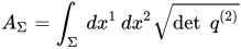
    From this we get the area of the surface Σ {\displaystyle \Sigma } {\displaystyle \Sigma } to be given by

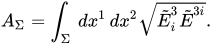
    A Σ = Σ d x 1 d x 2 det q ( 2 ) {\displaystyle A_{\Sigma }=\int _{\Sigma }\,dx^{1}\,dx^{2}{\sqrt {\det \;q^{(2)}}}} {\displaystyle A_{\Sigma }=\int _{\Sigma }\,dx^{1}\,dx^{2}{\sqrt {\det \;q^{(2)}}}}

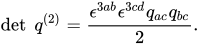
    where det q ( 2 ) = q 11 q 22 q 12 2 {\displaystyle \det q^{(2)}=q_{11}q_{22}-q_{12}^{2}} {\displaystyle \det q^{(2)}=q_{11}q_{22}-q_{12}^{2}} and is the determinant of the metric induced on Σ {\displaystyle \Sigma } {\displaystyle \Sigma }. This can be rewritten as

    det q ( 2 ) = ϵ 3 a b ϵ 3 c d q a c q b c 2 . {\displaystyle \det \;q^{(2)}={\epsilon ^{3ab}\epsilon ^{3cd}q_{ac}q_{bc} \over 2}.} {\displaystyle \det \;q^{(2)}={\epsilon ^{3ab}\epsilon ^{3cd}q_{ac}q_{bc} \over 2}.}

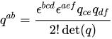
    The standard formula for an inverse matrix is

    q a b = ϵ b c d ϵ a e f q c e q d f 2 ! det ( q ) {\displaystyle q^{ab}={\epsilon ^{bcd}\epsilon ^{aef}q_{ce}q_{df} \over 2!\det(q)}} {\displaystyle q^{ab}={\epsilon ^{bcd}\epsilon ^{aef}q_{ce}q_{df} \over 2!\det(q)}}

    Note the similarity between this and the expression for det q ( 2 ) {\displaystyle \det q^{(2)}} {\displaystyle \det q^{(2)}}. But in Ashtekar variables we have E ~ i a E ~ b i = det ( q ) q a b {\displaystyle {\tilde {E}}_{i}^{a}{\tilde {E}}^{bi}=\det(q)q^{ab}} {\displaystyle {\tilde {E}}_{i}^{a}{\tilde {E}}^{bi}=\det(q)q^{ab}}. Therefore,

    A Σ = Σ d x 1 d x 2 E ~ i 3 E ~ 3 i . {\displaystyle A_{\Sigma }=\int _{\Sigma }\,dx^{1}\,dx^{2}{\sqrt {{\tilde {E}}_{i}^{3}{\tilde {E}}^{3i}}}.} {\displaystyle A_{\Sigma }=\int _{\Sigma }\,dx^{1}\,dx^{2}{\sqrt {{\tilde {E}}_{i}^{3}{\tilde {E}}^{3i}}}.}

    According to the rules of canonical quantization we should promote the triads E ~ i 3 {\displaystyle {\tilde {E}}_{i}^{3}} {\displaystyle {\tilde {E}}_{i}^{3}} to quantum operators,

    E ~ ^ i 3 δ δ A 3 i . {\displaystyle {\hat {\tilde {E}}}_{i}^{3}\sim {\delta \over \delta A_{3}^{i}}.} {\displaystyle {\hat {\tilde {E}}}_{i}^{3}\sim {\delta  \over \delta A_{3}^{i}}.}

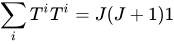
    It turns out that the area A Σ {\displaystyle A_{\Sigma }} {\displaystyle A_{\Sigma }} can be promoted to a well defined quantum operator despite the fact that we are dealing with product of two functional derivatives and worse we have a square-root to contend with as well.[5] Putting N = 2 J {\displaystyle N=2J} {\displaystyle N=2J}, we talk of being in the J-th representation. We note that i T i T i = J ( J + 1 ) 1 {\displaystyle \sum _{i}T^{i}T^{i}=J(J+1)1} {\displaystyle \sum _{i}T^{i}T^{i}=J(J+1)1}. This quantity is important in the final formula for the area spectrum. We simply state the result below,

    A ^ Σ W γ [ A ] = 8 π P l a n c k 2 β I j I ( j I + 1 ) W γ [ A ] {\displaystyle {\hat {A}}_{\Sigma }W_{\gamma }[A]=8\pi \ell _{Planck}^{2}\beta \sum _{I}{\sqrt {j_{I}(j_{I}+1)}}W_{\gamma }[A]} {\displaystyle {\hat {A}}_{\Sigma }W_{\gamma }[A]=8\pi \ell _{Planck}^{2}\beta \sum _{I}{\sqrt {j_{I}(j_{I}+1)}}W_{\gamma }[A]}

    where the sum is over all edges I {\displaystyle I} {\displaystyle I} of the Wilson loop that pierce the surface Σ {\displaystyle \Sigma } {\displaystyle \Sigma }.

    The formula for the volume of a region R {\displaystyle R} {\displaystyle R} is given by

    V = R d 3 x det ( q ) = 1 6 R d x 3 ϵ a b c ϵ i j k E ~ i a E ~ j b E ~ k c . {\displaystyle V=\int _{R}d^{3}x{\sqrt {\det(q)}}={1 \over 6}\int _{R}dx^{3}{\sqrt {\epsilon _{abc}\epsilon ^{ijk}{\tilde {E}}_{i}^{a}{\tilde {E}}_{j}^{b}{\tilde {E}}_{k}^{c}}}.} {\displaystyle V=\int _{R}d^{3}x{\sqrt {\det(q)}}={1 \over 6}\int _{R}dx^{3}{\sqrt {\epsilon _{abc}\epsilon ^{ijk}{\tilde {E}}_{i}^{a}{\tilde {E}}_{j}^{b}{\tilde {E}}_{k}^{c}}}.}

    The quantization of the volume proceeds the same way as with the area. As we take the derivative, and each time we do so we bring down the tangent vector γ ˙ a {\displaystyle {\dot {\gamma }}^{a}} {\displaystyle {\dot {\gamma }}^{a}}, when the volume operator acts on non-intersecting Wilson loops the result vanishes. Quantum states with non-zero volume must therefore involve intersections. Given that the anti-symmetric summation is taken over in the formula for the volume we would need at least intersections with three non-coplanar lines. Actually it turns out that one needs at least four-valent vertices for the volume operator to be non-vanishing.

    Mandelstam identities: su(2) Yang–Mills

    We now consider Wilson loops with intersections. We assume the real representation where the gauge group is S U ( 2 ) {\displaystyle SU(2)} {\displaystyle SU(2)}. Wilson loops are an over complete basis as there are identities relating different Wilson loops. These come about from the fact that Wilson loops are based on matrices (the holonomy) and these matrices satisfy identities, the so-called Mandelstam identities. Given any two S U ( 2 ) {\displaystyle SU(2)} {\displaystyle SU(2)} matrices A {\displaystyle \mathbb {A} } {\displaystyle \mathbb {A} } and B {\displaystyle \mathbb {B} } {\displaystyle \mathbb {B} } it is easy to check that,

    Tr ( A ) Tr ( B ) = Tr ( A B ) + Tr ( A B 1 ) . {\displaystyle \operatorname {Tr} (\mathbb {A} )\operatorname {Tr} (\mathbb {B} )=\operatorname {Tr} (\mathbb {A} \mathbb {B} )+\operatorname {Tr} (\mathbb {A} \mathbb {B} ^{-1}).} {\displaystyle \operatorname {Tr} (\mathbb {A} )\operatorname {Tr} (\mathbb {B} )=\operatorname {Tr} (\mathbb {A} \mathbb {B} )+\operatorname {Tr} (\mathbb {A} \mathbb {B} ^{-1}).}

    This implies that given two loops γ {\displaystyle \gamma } {\displaystyle \gamma } and η {\displaystyle \eta } {\displaystyle \eta } that intersect, we will have,

    W γ [ A ] W η [ A ] = W γ η [ A ] + W γ η 1 [ A ] {\displaystyle W_{\gamma }[A]W_{\eta }[A]=W_{\gamma \circ \eta }[A]+W_{\gamma \circ \eta ^{-1}}[A]} {\displaystyle W_{\gamma }[A]W_{\eta }[A]=W_{\gamma \circ \eta }[A]+W_{\gamma \circ \eta ^{-1}}[A]}

    where by η 1 {\displaystyle \eta ^{-1}} {\displaystyle \eta ^{-1}} we mean the loop η {\displaystyle \eta } {\displaystyle \eta } traversed in the opposite direction and γ η {\displaystyle \gamma \circ \eta } {\displaystyle \gamma \circ \eta } means the loop obtained by going around the loop γ {\displaystyle \gamma } {\displaystyle \gamma } and then along η {\displaystyle \eta } {\displaystyle \eta }. See figure below. This is called a Mandelstam identity of the second kind. There is the Mandelstam identity of the first kind W ( γ 1 γ 2 ) = W ( γ 2 γ 1 ) {\displaystyle W(\gamma _{1}\circ \gamma _{2})=W(\gamma _{2}\circ \gamma _{1})} {\displaystyle W(\gamma _{1}\circ \gamma _{2})=W(\gamma _{2}\circ \gamma _{1})}. Spin networks are certain linear combinations of intersecting Wilson loops designed to address the over-completeness introduced by the Mandelstam identities.

    Loop representation in gauge theories and quantum gravity
    Graphical representation of the Mandestam identity relating different Wilson loops.

    Spin network states

    In fact spin networks constitute a basis for all gauge invariant functions which minimize the degree of over-completeness of the loop basis, and for trivalent intersections eliminate it entirely.

    As mentioned above the holonomy tells you how to propagate test spin half particles. A spin network state assigns an amplitude to a set of spin half particles tracing out a path in space, merging and splitting. These are described by spin networks γ {\displaystyle \gamma } {\displaystyle \gamma }: the edges are labelled by spins together with `intertwiners’ at the vertices which are prescription for how to sum over different ways the spins are rerouted. The sum over rerouting are chosen as such to make the form of the intertwiner invariant under Gauss gauge transformations.

    Uniqueness of the loop representation in LQG

    Theorems establishing the uniqueness of the loop representation as defined by Ashtekar et al. (i.e. a certain concrete realization of a Hilbert space and associated operators reproducing the correct loop algebra – the realization that everybody was using) have been given by two groups (Lewandowski, Okolow, Sahlmann and Thiemann)[6] and (Christian Fleischhack).[7] Before this result was established it was not known whether there could be other examples of Hilbert spaces with operators invoking the same loop algebra, other realizations, not equivalent to the one that had been used so far.

    Knot theory and loops in topological field theory

    A common method of describing a knot (or link, which are knots of several components entangled with each other) is to consider its projected image onto a plane called a knot diagram. Any given knot (or link) can be drawn in many different ways using a knot diagram. Therefore, a fundamental problem in knot theory is determining when two descriptions represent the same knot. Given a knot diagram, one tries to find a way to assign a knot invariant to it, sometimes a polynomial – called a knot polynomial. Two knot diagrams with different polynomials generated by the same procedure necessarily correspond to different knots. However, if the polynomials are the same, it may not mean that they correspond to the same knot. The better a polynomial is at distinguishing knots the more powerful it is.
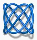
    In 1984, Jones [8] announced the discovery of a new link invariant, which soon led to a bewildering profusion of generalizations. He had found a new knot polynomial, the Jones polynomial. Specifically, it is an invariant of an oriented knot or link which assigns to each oriented knot or link a polynomial with integer coefficients.

    In the late 1980s, Witten coined the term topological quantum field theory for a certain type of physical theory in which the expectation values of observable quantities are invariant under diffeomorphisms.

    Witten [9] gave a heuristic derivation of the Jones polynomial and its generalizations from Chern–Simons theory. The basic idea is simply that the vacuum expectation values of Wilson loops in Chern–Simons theory are link invariants because of the diffeomorphism-invariance of the theory. To calculate these expectation values, however, Witten needed to use the relation between Chern–Simons theory and a conformal field theory known as the Wess–Zumino–Witten model (or the WZW model).

    References

    1. Jacobson, Ted; Smolin, Lee (4 April 1988). “Nonperturbative quantum geometries”. Nuclear Physics B. 299 (2): 295–345. doi:10.1016/0550-3213(88)90286-6. ISSN 0550-3213.
    2. Witten, Edward (1989). “Quantum field theory and the Jones polynomial”. Communications in Mathematical Physics. 121 (3): 351–399. Bibcode:1989CMaPh.121..351W. doi:10.1007/bf01217730. ISSN 0010-3616. S2CID 14951363.
    3. Giles, R. (1981-10-15). “Reconstruction of gauge potentials from Wilson loops”. Physical Review D. 24 (8): 2160–2168. Bibcode:1981PhRvD..24.2160G. doi:10.1103/physrevd.24.2160. ISSN 0556-2821.
    4. Rovelli, Carlo; Smolin, Lee (1988-09-05). “Knot Theory and Quantum Gravity”. Physical Review Letters. 61 (10): 1155–1158. Bibcode:1988PhRvL..61.1155R. doi:10.1103/physrevlett.61.1155. ISSN 0031-9007. PMID 10038716.
    5. For example see section 8.2 of A First Course in Loop Quantum Gravity, Gambini, R, and Pullin, J. Published by Oxford University Press 2011.
    6. Lewandowski, Jerzy; Okołów, Andrzej; Sahlmann, Hanno; Thiemann, Thomas (2006-08-22). “Uniqueness of Diffeomorphism Invariant States on Holonomy–Flux Algebras”. Communications in Mathematical Physics. 267 (3): 703–733. arXiv:gr-qc/0504147. Bibcode:2006CMaPh.267..703L. doi:10.1007/s00220-006-0100-7. ISSN 0010-3616. S2CID 14866220.
    7. Fleischhack, Christian (2006-08-11). “Irreducibility of the Weyl Algebra in Loop Quantum Gravity”. Physical Review Letters. 97 (6) 061302. Bibcode:2006PhRvL..97f1302F. doi:10.1103/physrevlett.97.061302. ISSN 0031-9007. PMID 17026156.
    8. V. Jones, A polynomial invariant for knots via von Neumann algebras, reprinted
      in New Developments in the Theory of Knots, ed. T. Kohno, World Scientific, Singapore, 1989.
    9. Witten, E. (1989). “Quantum field theory and the Jones polynomial”. Communications in Mathematical Physics. 121 (3): 351–399. Bibcode:1989CMaPh.121..351W. doi:10.1007/BF01217730. MR 0990772. S2CID 14951363.


    This article is adapted from “Loop representation in gauge theories and quantum gravity” on Wikipedia, written by its contributors, and used under CC BY-SA 4.0. Text on this page is available under the same licence. Source snapshot: Wikipedia via Kiwix, 2026-07-20.

  • Loop braid group

    The loop braid group is a mathematical group structure that is used in some models of theoretical physics to model the exchange of particles with loop-like topologies within three dimensions of space and time.

    The basic operations which generate a loop braid group for n loops are exchanges of two adjacent loops, and passing one adjacent loop through another. The topology forces these generators to satisfy some relations, which determine the group.

    To be precise, the loop braid group on n loops is defined as the motion group of n disjoint circles embedded in a compact three-dimensional “box” diffeomorphic to the three-dimensional disk. A motion is a loop in the configuration space, which consists of all possible ways of embedding n circles into the 3-disk. This becomes a group in the same way as loops in any space can be made into a group; first, we define equivalence classes of loops by letting paths g and h be equivalent iff they are related by a (smooth) homotopy, and then we define a group operation on the equivalence classes by concatenation of paths. In his 1962 Ph.D. thesis, David M. Dahm was able to show that there is an injective homomorphism from this group into the automorphism group of the free group on n generators, so it is natural to identify the group with this subgroup of the automorphism group.[1] One may also show that the loop braid group is isomorphic to the welded braid group, as is done for example in a paper by John C. Baez, Derek Wise, and Alissa Crans, which also gives some presentations of the loop braid group using the work of Xiao-Song Lin.[2]

    See also

    References

    1. Goldsmith, Deborah L. (1981), “The theory of motion groups”, The Michigan Mathematical Journal, 28 (1): 3–17, doi:10.1307/mmj/1029002454, MR 0600411.
    2. Baez, John C.; Wise, Derek K.; Crans, Alissa S. (2007), “Exotic statistics for strings in 4D BF theory”, Advances in Theoretical and Mathematical Physics, 11 (5): 707–749, arXiv:gr-qc/0603085, Bibcode:2006gr.qc…..3085B, doi:10.4310/atmp.2007.v11.n5.a1, MR 2362007.


    This article is adapted from “Loop braid group” on Wikipedia, written by its contributors, and used under CC BY-SA 4.0. Text on this page is available under the same licence. Source snapshot: Wikipedia via Kiwix, 2026-07-20.

  • Lobster buoy hitch

    Lobster buoy hitch
    Lobster buoy hitch
    Category Hitch
    Related Cow hitch, Buntline hitch, Two half-hitches
    Releasing Jamming
    Typical use attaching lines to rings, eyes, posts, rods, and railings
    ABoK #58, #1714, #1839
    Lobster buoy hitch
    Untightened Lobster buoy hitch

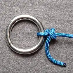
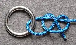
    The lobster buoy hitch is similar to the buntline hitch, but made with a cow hitch around the standing part rather than a clove hitch.

    Like the buntline hitch, this knot is strong, secure and compact.

    See also

    References

    • Clifford W. Ashley. The Ashley Book of Knots. Doubleday, New York. #1714, p. 295. ISBN 0-571-09659-X


    This article is adapted from “Lobster buoy hitch” on Wikipedia, written by its contributors, and used under CC BY-SA 4.0. Text on this page is available under the same licence. Source snapshot: Wikipedia via Kiwix, 2026-07-20.

  • List of prime knots


    In knot theory, prime knots are those knots that are indecomposable under the operation of knot sum. The prime knots with ten or fewer crossings are listed here for quick comparison of their properties and varied naming schemes.

    Table of prime knots

    Six or fewer crossings

    Name Picture Alexander–
    Briggs

    Rolfsen
    Dowker–
    Thistlethwaite
    Dowker
    notation
    Conway
    notation
    crossinglist
    Unknot List of prime knots 01 0a1 0
    Trefoil knot List of prime knots 31 3a1 4 6 2 [3] 123:123
    Figure-eight knot List of prime knots 41 4a1 4 6 8 2 [22] 1234:2143

    1231\4324

    Cinquefoil knot List of prime knots 51 5a2 6 8 10 2 4 [5] 12345:12345
    Three-twist knot List of prime knots 52 5a1 4 8 10 2 6 [32] 12345:12543

    1231\452354

    Stevedore knot List of prime knots 61 6a3 4 8 12 10 2 6 [42] 123456:216543

    1231\45632654

    62 knot List of prime knots 62 6a2 4 8 10 12 2 6 [312] 123456:234165

    1231\45632456

    63 knot List of prime knots 63 6a1 4 8 10 2 12 6 [2112] 123456:236145

    1231\45642356

    1231\45236456

    Seven crossings

    Picture Alexander–
    Briggs–
    Rolfsen
    Dowker–
    Thistlethwaite
    Dowker
    notation
    Conway
    notation
    crossinglist
    List of prime knots 71 7a7 8 10 12 14 2 4 6 [7] 1-7:1-7
    List of prime knots 72 7a4 4 10 14 12 2 8 6 [52] 1-7:127-3
    List of prime knots 73 7a5 6 10 12 14 2 4 8 [43]
    List of prime knots 74 7a6 6 10 12 14 4 2 8 [313]
    List of prime knots 75 7a3 4 10 12 14 2 8 6 [322]
    List of prime knots 76 7a2 4 8 12 2 14 6 10 [2212]
    List of prime knots 77 7a1 4 8 10 12 2 14 6 [21112]

    Eight crossings

    Picture Alexander–
    Briggs–
    Rolfsen
    Dowker–
    Thistlethwaite
    Dowker
    notation
    Conway
    notation
    List of prime knots 81 8a­11 4 10 16 14 12 2 8 6 [62]
    List of prime knots 82 8a8 4 10 12 14 16 2 6 8 [512]
    List of prime knots 83 8a­18 6 12 10 16 14 4 2 8 [44]
    List of prime knots 84 8a­17 6 10 12 16 14 4 2 8 [413]
    List of prime knots 85 8a­13 6 8 12 2 14 16 4 10 [3,3,2]
    List of prime knots 86 8a­10 4 10 14 16 12 2 8 6 [332]

    List of prime knots

    87 8a6 4 10 12 14 2 16 6 8 [4112]

    List of prime knots

    88 8a4 4 8 12 2 16 14 6 10 [2312]

    List of prime knots

    89 8a­16 6 10 12 14 16 4 2 8 [3113]

    List of prime knots

    810 8a3 4 8 12 2 14 16 6 10 [3,21,2]

    List of prime knots

    811 8a9 4 10 12 14 16 2 8 6 [3212]
    List of prime knots 812 8a5 4 8 14 10 2 16 6 12 [2222]

    List of prime knots

    813 8a7 4 10 12 14 2 16 8 6 [31112]

    List of prime knots

    814 8a1 4 8 10 14 2 16 6 12 [22112]
    List of prime knots 815 8a2 4 8 12 2 14 6 16 10 [21,21,2]
    List of prime knots 816 8a­15 6 8 14 12 4 16 2 10 [.2.20]
    List of prime knots 817 8a­14 6 8 12 14 4 16 2 10 [.2.2]
    List of prime knots 818 8a­12 6 8 10 12 14 16 2 4 [8*]
    List of prime knots 819 8n3 4 8 -12 2 -14 -16 -6 -10 [3,3,2-]
    List of prime knots 820 8n1 4 8 -12 2 -14 -6 -16 -10 [3,21,2-]
    List of prime knots 821 8n2 4 8 -12 2 14 -6 16 10 [21,21,2-]

    Nine crossings

    Picture Alexander–
    Briggs–
    Rolfsen
    Dowker–
    Thistlethwaite
    Dowker
    notation
    Conway
    notation
    List of prime knots 91 9a­41 10 12 14 16 18 2 4 6 8 [9]
    List of prime knots 92 9a­27 4 12 18 16 14 2 10 8 6 [72]
    List of prime knots 93 9a­38 8 12 14 16 18 2 4 6 10 [63]
    List of prime knots 94 9a­35 6 12 14 18 16 2 4 10 8 [54]

    List of prime knots

    95 9a­36 6 12 14 18 16 4 2 10 8 [513]

    List of prime knots

    96 9a­23 4 12 14 16 18 2 10 6 8 [522]

    List of prime knots

    97 9a­26 4 12 16 18 14 2 10 8 6 [342]

    List of prime knots

    98 9a8 4 8 14 2 18 16 6 12 10 [2412]

    List of prime knots

    99 9a­33 6 12 14 16 18 2 4 10 8 [423]

    List of prime knots

    910 9a­39 8 12 14 16 18 2 6 4 10 [333]

    List of prime knots

    911 9a­20 4 10 14 16 12 2 18 6 8 [4122]
    List of prime knots 912 9a­22 4 10 16 14 2 18 8 6 12 [4212]
    List of prime knots 913 9a­34 6 12 14 16 18 4 2 10 8 [3213]
    List of prime knots 914 9a­17 4 10 12 16 14 2 18 8 6 [41112]
    List of prime knots 915 9a­10 4 8 14 10 2 18 16 6 12 [2322]
    List of prime knots 916 9a­25 4 12 16 18 14 2 8 10 6 [3,3,2+]
    List of prime knots 917 9a­14 4 10 12 14 16 2 6 18 8 [21312]
    List of prime knots 918 9a­24 4 12 14 16 18 2 10 8 6 [3222]
    List of prime knots 919 9a3 4 8 10 14 2 18 16 6 12 [23112]

    List of prime knots

    920 9a­19 4 10 14 16 2 18 8 6 12 [31212]

    List of prime knots

    921 9a­21 4 10 14 16 12 2 18 8 6 [31122]

    List of prime knots

    922 9a2 4 8 10 14 2 16 18 6 12 [211,3,2]
    List of prime knots 923 9a­16 4 10 12 16 2 8 18 6 14 [22122]

    List of prime knots

    924 9a7 4 8 14 2 16 18 6 12 10 [3,21,2+]

    List of prime knots

    925 9a4 4 8 12 2 16 6 18 10 14 [22,21,2]

    List of prime knots

    926 9a­15 4 10 12 14 16 2 18 8 6 [311112]

    List of prime knots

    927 9a­12 4 10 12 14 2 18 16 6 8 [212112]

    List of prime knots

    928 9a5 4 8 12 2 16 14 6 18 10 [21,21,2+]

    List of prime knots

    929 9a­31 6 10 14 18 4 16 8 2 12 [.2.20.2]

    List of prime knots

    930 9a1 4 8 10 14 2 16 6 18 12 [211,21,2]

    List of prime knots

    931 9a­13 4 10 12 14 2 18 16 8 6 [2111112]

    List of prime knots

    932 9a6 4 8 12 14 2 16 18 10 6 [.21.20]

    List of prime knots

    933 9a­11 4 8 14 12 2 16 18 10 6 [.21.2]

    List of prime knots

    934 9a­28 6 8 10 16 14 18 4 2 12 [8*20]
    List of prime knots 935 9a­40 8 12 16 14 18 4 2 6 10 [3,3,3]

    List of prime knots

    936 9a9 4 8 14 10 2 16 18 6 12 [22,3,2]

    List of prime knots

    937 9a­18 4 10 14 12 16 2 6 18 8 [3,21,21]

    List of prime knots

    938 9a­30 6 10 14 18 4 16 2 8 12 [.2.2.2]

    List of prime knots

    939 9a­32 6 10 14 18 16 2 8 4 12 [2:2:20]
    List of prime knots 940 9a­27 6 16 14 12 4 2 18 10 8 [9*]
    List of prime knots 941 9a­29 6 10 14 12 16 2 18 4 8 [20:20:20]

    List of prime knots

    942 9n4 4 8 10 14 2 16 18 6 12 [22,3,2]

    List of prime knots

    943 9n3 4 8 10 14 2 16 6 18 12 [211,3,2]

    List of prime knots

    944 9n1 4 8 10 14 2 16 6 18 12 [22,21,2]

    List of prime knots

    945 9n2 4 8 10 14 2 16 6 18 12 [211,21,2]

    List of prime knots

    946 9n5 4 10 14 12 16 2 6 18 8 [3,3,21]
    List of prime knots 947 9n7 6 8 10 16 14 18 4 2 12 [8*-20]

    List of prime knots

    948 9n6 4 10 14 12 16 2 6 18 8 [21,21,21]

    List of prime knots

    949 9n8 6 -10 14 12 16 2 18 4 8 [20:20:20]

    Ten crossings

    Picture Alexander–
    Briggs–
    Rolfsen
    Dowker–
    Thistlethwaite
    Dowker
    notation
    Conway
    notation
    101 10a­75 4 12 20 18 16 14 2 10 8 6 [82]
    102 10a­59 4 12 14 16 18 20 2 6 8 10 [712]
    103 10a­­117 6 14 12 20 18 16 4 2 10 8 [64]
    104 10a­­113 6 12 14 20 18 16 4 2 10 8 [613]
    105 10a­56 4 12 14 16 18 2 20 6 8 10 [6112]
    106 10a­70 4 12 16 18 20 14 2 10 6 8 [532]
    107 10a­65 4 12 14 18 16 20 2 10 8 6 [5212]
    108 10a­­114 6 14 12 16 18 20 4 2 8 10 [514]
    109 10a­­110 6 12 14 16 18 20 4 2 8 10 [5113]
    1010 10a­64 4 12 14 18 16 2 20 10 8 6 [51112]
    1011 10a­­116 6 14 12 18 20 16 4 2 10 8 [433]
    1012 10a­43 4 10 14 16 2 20 18 6 8 12 [4312]
    1013 10a­54 4 10 18 16 12 2 20 8 6 14 [4222]
    1014 10a­33 4 10 12 16 18 2 20 6 8 14 [42112]
    1015 10a­68 4 12 16 18 14 2 10 20 6 8 [4132]
    1016 10a­­115 6 14 12 16 18 20 4 2 10 8 [4123]
    1017 10a­­107 6 12 14 16 18 2 4 20 8 10 [4114]
    1018 10a­63 4 12 14 18 16 2 10 20 8 6 [41122]
    1019 10a­­108 6 12 14 16 18 2 4 20 10 8 [41113]
    1020 10a­74 4 12 18 20 16 14 2 10 8 6 [352]
    1021 10a­60 4 12 14 16 18 20 2 6 10 8 [3412]
    1022 10a­­112 6 12 14 18 20 16 4 2 10 8 [3313]
    1023 10a­57 4 12 14 16 18 2 20 6 10 8 [33112]
    1024 10a­71 4 12 16 18 20 14 2 10 8 6 [3232]
    List of prime knots 1025 10a­61 4 12 14 16 18 20 2 10 8 6 [32212]
    1026 10a­­111 6 12 14 16 18 20 4 2 10 8 [32113]
    1027 10a­58 4 12 14 16 18 2 20 10 8 6 [321112]
    1028 10a­44 4 10 14 16 2 20 18 8 6 12 [31312]
    1029 10a­53 4 10 16 18 12 2 20 8 6 14 [31222]
    1030 10a­34 4 10 12 16 18 2 20 8 6 14 [312112]
    1031 10a­69 4 12 16 18 14 2 10 20 8 6 [31132]
    1032 10a­55 4 12 14 16 18 2 10 20 8 6 [311122]
    1033 10a­­109 6 12 14 16 18 4 2 20 10 8 [311113]
    1034 10a­19 4 8 14 2 20 18 16 6 12 10 [2512]
    1035 10a­23 4 8 16 10 2 20 18 6 14 12 [2422]
    1036 10a5 4 8 10 16 2 20 18 6 14 12 [24112]
    1037 10a­49 4 10 16 12 2 8 20 18 6 14 [2332]
    1038 10a­29 4 10 12 16 2 8 20 18 6 14 [23122]
    1039 10a­26 4 10 12 14 18 2 6 20 8 16 [22312]
    1040 10a­30 4 10 12 16 2 20 6 18 8 14 [222112]
    1041 10a­35 4 10 12 16 20 2 8 18 6 14 [221212]
    1042 10a­31 4 10 12 16 2 20 8 18 6 14 [2211112]
    1043 10a­52 4 10 16 14 2 20 8 18 6 12 [212212]
    1044 10a­32 4 10 12 16 14 2 20 18 8 6 [2121112]
    1045 10a­25 4 10 12 14 16 2 20 18 8 6 [21111112]
    1046 10a­81 6 8 14 2 16 18 20 4 10 12 [5,3,2]
    1047 10a­15 4 8 14 2 16 18 20 6 10 12 [5,21,2]
    1048 10a­79 6 8 14 2 16 18 4 20 10 12 [41,3,2]
    1049 10a­13 4 8 14 2 16 18 6 20 10 12 [41,21,2]
    1050 10a­82 6 8 14 2 16 18 20 4 12 10 [32,3,2]
    1051 10a­16 4 8 14 2 16 18 20 6 12 10 [32,21,2]
    1052 10a­80 6 8 14 2 16 18 4 20 12 10 [311,3,2]
    1053 10a­14 4 8 14 2 16 18 6 20 12 10 [311,21,2]
    1054 10a­48 4 10 16 12 2 8 18 20 6 14 [23,3,2]
    1055 10a9 4 8 12 2 16 6 20 18 10 14 [23,21,2]
    1056 10a­28 4 10 12 16 2 8 18 20 6 14 [221,3,2]
    1057 10a6 4 8 12 2 14 18 6 20 10 16 [221,21,2]
    1058 10a­20 4 8 14 10 2 18 6 20 12 16 [22,22,2]
    List of prime knots 1059 10a2 4 8 10 14 2 18 6 20 12 16 [22,211,2]
    List of prime knots 1060 10a1 4 8 10 14 2 16 18 6 20 12 [211,211,2]
    1061 10a­­123 8 10 16 14 2 18 20 6 4 12 [4,3,3]
    1062 10a­41 4 10 14 16 2 18 20 6 8 12 [4,3,21]
    1063 10a­51 4 10 16 14 2 18 8 6 20 12 [4,21,21]
    1064 10a­­122 8 10 14 16 2 18 20 6 4 12 [31,3,3]
    1065 10a­42 4 10 14 16 2 18 20 8 6 12 [31,3,21]
    1066 10a­40 4 10 14 16 2 18 8 6 20 12 [31,21,21]
    1067 10a­37 4 10 14 12 18 2 6 20 8 16 [22,3,21]
    1068 10a­67 4 12 16 14 18 2 20 6 10 8 [211,3,3]
    1069 10a­38 4 10 14 12 18 2 16 6 20 8 [211,21,21]
    1070 10a­22 4 8 16 10 2 18 20 6 14 12 [22,3,2+]
    1071 10a­10 4 8 12 2 18 14 6 20 10 16 [22,21,2+]
    1072 10a4 4 8 10 16 2 18 20 6 14 12 [211,3,2+]
    1073 10a3 4 8 10 14 2 18 16 6 20 12 [211,21,2+]
    1074 10a­62 4 12 14 16 20 18 2 8 6 10 [3,3,21+]
    List of prime knots 1075 10a­27 4 10 12 14 18 2 16 6 20 8 [21,21,21+]
    1076 10a­73 4 12 18 20 14 16 2 10 8 6 [3,3,2++]
    1077 10a­18 4 8 14 2 18 20 16 6 12 10 [3,21,2++]
    1078 10a­17 4 8 14 2 18 16 6 12 20 10 [21,21,2++]
    1079 10a­78 6 8 12 2 16 4 18 20 10 14 [(3,2)(3,2)]
    1080 10a8 4 8 12 2 16 6 18 20 10 14 [(3,2)(21,2)]
    1081 10a7 4 8 12 2 16 6 18 10 20 14 [(21,2)(21,2)]
    1082 10a­83 6 8 14 16 4 18 20 2 10 12 [.4.2]
    1083 10a­84 6 8 16 14 4 18 20 2 12 10 [.31.20]
    1084 10a­50 4 10 16 14 2 8 18 20 12 6 [.22.2]
    1085 10a­86 6 8 16 14 4 18 20 2 10 12 [.4.20]
    1086 10a­87 6 8 14 16 4 18 20 2 12 10 [.31.2]
    1087 10a­39 4 10 14 16 2 8 18 20 12 6 [.22.20]
    1088 10a­11 4 8 12 14 2 16 20 18 10 6 [.21.21]
    1089 10a­21 4 8 14 12 2 16 20 18 10 6 [.21.210]
    1090 10a­92 6 10 14 2 16 20 18 8 4 12 [.3.2.2]
    1091 10a­­106 6 10 20 14 16 18 4 8 2 12 [.3.2.20]
    1092 10a­46 4 10 14 18 2 16 8 20 12 6 [.21.2.20]
    1093 10a­­101 6 10 16 20 14 4 18 2 12 8 [.3.20.2]
    1094 10a­91 6 10 14 2 16 18 20 8 4 12 [.30.2.2]
    1095 10a­47 4 10 14 18 2 16 20 8 12 6 [.210.2.2]
    1096 10a­24 4 8 18 12 2 16 20 6 10 14 [.2.21.2]
    1097 10a­12 4 8 12 18 2 16 20 6 10 14 [.2.210.2]
    1098 10a­96 6 10 14 18 2 16 20 4 8 12 [.2.2.2.20]
    1099 10a­­103 6 10 18 14 2 16 20 8 4 12 [.2.2.20.20]
    10100 10a­­104 6 10 18 14 16 4 20 8 2 12 [3:2:2]
    10101 10a­45 4 10 14 18 2 16 6 20 8 12 [21:2:2]
    10102 10a­97 6 10 14 18 16 4 20 2 8 12 [3:2:20]
    10103 10a­­105 6 10 18 16 14 4 20 8 2 12 [30:2:2]
    10104 10a­­118 6 16 12 14 18 4 20 2 8 10 [3:20:20]
    10105 10a­72 4 12 16 20 18 2 8 6 10 14 [21:20:20]
    10106 10a­95 6 10 14 16 18 4 20 2 8 12 [30:2:20]
    10107 10a­66 4 12 16 14 18 2 8 20 10 6 [210:2:20]
    10108 10a­­119 6 16 12 14 18 4 20 2 10 8 [30:20:20]
    10109 10a­93 6 10 14 16 2 18 4 20 8 12 [2.2.2.2]
    10110 10a­­100 6 10 16 20 14 2 18 4 8 12 [2.2.2.20]
    10111 10a­98 6 10 16 14 2 18 8 20 4 12 [2.2.20.2]
    10112 10a­76 6 8 10 14 16 18 20 2 4 12 [8*3]
    10113 10a­36 4 10 14 12 2 16 18 20 8 6 [8*21]
    10114 10a­77 6 8 10 14 16 20 18 2 4 12 [8*30]
    10115 10a­94 6 10 14 16 4 18 2 20 12 8 [8*20.20]
    List of prime knots 10116 10a­­120 6 16 18 14 2 4 20 8 10 12 [8*2:2]
    10117 10a­99 6 10 16 14 18 4 20 2 12 8 [8*2:20]
    10118 10a­88 6 8 18 14 16 4 20 2 10 12 [8*2:.2]
    10119 10a­85 6 8 14 18 16 4 20 10 2 12 [8*2:.20]
    List of prime knots 10120 10a­­102 6 10 18 12 4 16 20 8 2 14 [8*20::20]
    10121 10a­90 6 10 12 20 18 16 8 2 4 14 [9*20]
    List of prime knots 10122 10a­89 6 10 12 14 18 16 20 2 4 8 [9*.20]
    List of prime knots 10123 10a­­121 8 10 12 14 16 18 20 2 4 6 [10*]
    10124 10n­21 4 8 -14 2 -16 -18 -20 -6 -10 -12 [5,3,2-]
    10125 10n­15 4 8 14 2 -16 -18 6 -20 -10 -12 [5,21,2-]
    10126 10n­17 4 8 -14 2 -16 -18 -6 -20 -10 -12 [41,3,2-]
    10127 10n­16 4 8 -14 2 16 18 -6 20 10 12 [41,21,2-]
    10128 10n­22 4 8 -14 2 -16 -18 -20 -6 -12 -10 [32,3,2-]
    10129 10n­18 4 8 14 2 -16 -18 6 -20 -12 -10 [32,21,-2]
    10130 10n­20 4 8 -14 2 -16 -18 -6 -20 -12 -10 [311,3,2-]
    10131 10n­19 4 8 -14 2 16 18 -6 20 12 10 [311,21,2-]
    List of prime knots 10132 10n­13 4 8 -12 2 -16 -6 -20 -18 -10 -14 [23,3,2-]
    10133 10n4 4 8 12 2 -14 -18 6 -20 -10 -16 [23,21,2-]
    10134 10n6 4 8 -12 2 -14 -18 -6 -20 -10 -16 [221,3,2-]
    10135 10n5 4 8 -12 2 14 18 -6 20 10 16 [221,21,2-]
    10136 10n3 4 8 10 -14 2 -18 -6 -20 -12 -16 [22,22,2-]
    10137 10n2 4 8 10 -14 2 -16 -18 -6 -20 -12 [22,211,2-]
    10138 10n1 4 8 10 -14 2 16 18 -6 20 12 [211,211,2-]
    10139 10n­27 4 10 -14 -16 2 -18 -20 -6 -8 -12 [4,3,3-]
    10140 10n­29 4 10 -14 -16 2 18 20 -8 -6 12 [4,3,21-]
    10141 10n­25 4 10 -14 -16 2 18 -8 -6 20 12 [4,21,21-]
    10142 10n­30 4 10 -14 -16 2 -18 -20 -8 -6 -12 [31,3,3-]
    10143 10n­26 4 10 -14 -16 2 -18 -8 -6 -20 -12 [31,3,21-]
    10144 10n­28 4 10 14 16 2 -18 -20 8 6 -12 [31,21,21-]
    10145 10n­14 4 8 -12 -18 2 -16 -20 -6 -10 -14 [22,3,3-]
    10146 10n­23 4 8 -18 -12 2 -16 -20 -6 -10 -14 [22,21,21-]
    10147 10n­24 4 10 -14 12 2 16 18 -20 8 -6 [211,3,21-]
    10148 10n­12 4 8 -12 2 -16 -6 -18 -20 -10 -14 [(3,2)(3,2-)]
    10149 10n­11 4 8 -12 2 16 -6 18 20 10 14 [(3,2)(21,2-)]
    10150 10n9 4 8 -12 2 -16 -6 -18 -10 -20 -14 [(21,2)(3,2-)]
    10151 10n8 4 8 -12 2 16 -6 18 10 20 14 [(21,2)(21,2-)]
    10152 10n­36 6 8 12 2 -16 4 -18 -20 -10 -14 [(3,2)-(3,2)]
    10153 10n­10 4 8 12 2 -16 6 -18 -20 -10 -14 [(3,2)-(21,2)]
    10154 10n7 4 8 12 2 -16 6 -18 -10 -20 -14 [(21,2)-(21,2)]
    10155 10n­39 6 10 14 16 18 4 -20 2 8 -12 [-3:2:2]
    10156 10n­32 4 12 16 -14 18 2 -8 20 10 6 [-3:2:20]
    10157 10n­42 6 -10 -18 14 -2 -16 20 8 -4 12 [-3:20:20]
    10158 10n­41 6 -10 -16 14 -2 -18 8 20 -4 -12 [-30:2:2]
    10159 10n­34 6 8 10 14 16 -18 -20 2 4 -12 [-30:2:20]
    10160 10n­33 4 12 -16 -14 -18 2 -8 -20 -10 -6 [-30:20:20]
    List of prime knots 10161[a] 10n­31 4 12 -16 14 -18 2 8 -20 -10 -6 [3:-20:-20]
    10162[b] 10n­40 6 10 14 18 16 4 -20 2 8 -12 [-30:-20:-20]
    10163[c] 10n­35 6 8 10 14 16 -20 -18 2 4 -12 [8*-30]
    10164[d] 10n­38 6 -10 -12 14 -18 -16 20 -2 -4 -8 [8*2:-20]
    10165[e] 10n­37 6 8 14 18 16 4 -20 10 2 -12 [8*2:.-20]

    Higher

    List of prime knots
    Kinoshita–Terasaka & Conway knots

    Table of prime links

    Eight or fewer crossings

    Name Picture Alexander–
    Briggs

    Rolfsen
    Dowker–
    Thistlethwaite
    Dowker
    notation
    Conway
    notation
    Unlink List of prime knots 02
    1
    Hopf link List of prime knots 22
    1
    L2a1 [2]
    Solomon’s
    knot
    List of prime knots 42
    1
    L4a1 [4]
    Whitehead
    link
    List of prime knots 52
    1
    L5a1 [212]
    L6a1 62
    3
    L6a1
    L6a2 62
    2
    L6a2
    L6a3 62
    1
    L6a3
    Borromean
    rings
    List of prime knots 63
    2
    L6a4 [.1]
    L6a5 63
    1
    L6a5
    L6n1 List of prime knots 63
    3
    L6n1
    L7a1 72
    6
    L7a1
    L7a2 72
    5
    L7a2
    L7a3 72
    4
    L7a3
    L7a4 72
    3
    L7a4
    L7a5 72
    2
    L7a5
    L7a6 72
    1
    L7a6
    L7a7 73
    1
    L7a7
    L7n1 72
    7
    L7n1
    L7n2 72
    8
    L7n2 (6,-8|-10,12,-14,2,-4)

    Higher

    List of prime knots
    (36,3)-torus link
    Picture Alexander–
    Briggs–
    Rolfsen
    Dowker–
    Thistlethwaite
    Dowker
    notation
    Conway
    notation
    List of prime knots 82
    1
    L8a14
    List of prime knots L10a140 [.3:30]

    See also

    Notes

    1. Originally listed as both 10161 and 10162 in the Rolfsen table. The error was discovered by Kenneth Perko (see Perko pair).
    2. Listed as 10163 in the Rolfsen table.
    3. Listed as 10164 in the Rolfsen table.
    4. Listed as 10165 in the Rolfsen table.
    5. Listed as 10166 in the Rolfsen table.

    External links


    This article is adapted from “List of prime knots” on Wikipedia, written by its contributors, and used under CC BY-SA 4.0. Text on this page is available under the same licence. Source snapshot: Wikipedia via Kiwix, 2026-07-20.

  • List of mathematical knots and links

    List of mathematical knots and links
    A table of all prime knots with seven crossings or fewer (not including mirror images).

    This article contains a list of mathematical knots and links. See also list of knots, list of geometric topology topics.

    Knots

    Prime knots

    • 01 knot/Unknot – a simple un-knotted closed loop
    • 31 knot/Trefoil knot – (2,3)-torus knot, the two loose ends of a common overhand knot joined together
    • 41 knot/Figure-eight knot (mathematics) – a prime knot with a crossing number four
    • 51 knot/Cinquefoil knot, (5,2)-torus knot, Solomon’s seal knot, pentafoil knot – a prime knot with crossing number five which can be arranged as a {5/2} star polygon (pentagram)
    • 52 knot/Three-twist knot – the twist knot with three-half twists
    • 61 knot/Stevedore knot (mathematics) – a prime knot with crossing number six, it can also be described as a twist knot with four twists
    • 62 knot – a prime knot with crossing number six
    • 63 knot – a prime knot with crossing number six
    • 71 knot, septafoil knot, (7,2)-torus knot – a prime knot with crossing number seven, which can be arranged as a {7/2} star polygon (heptagram)
    • 74 knot, “endless knot”
    • 818 knot, “carrick mat”
    • 10161/10162, known as the Perko pair; this was a single knot listed twice in Dale Rolfsen’s knot table; the duplication was discovered by Kenneth Perko
    • 12n242/(−2,3,7) pretzel knot
    • (p, q)-torus knot – a special kind of knot that lies on the surface of an unknotted torus in R3

    Composite

    Links

    • 02
      1
      link/Unlink – equivalent under ambient isotopy to finitely many disjoint circles in the plane
    • 22
      1
      link/Hopf link – the simplest nontrivial link with more than one component; it consists of two circles linked together exactly once (L2a1)
    • 42
      1
      link/Solomon’s knot (a two component “link” rather than a one component “knot”) – a traditional decorative motif used since ancient times (L4a1)
    • 52
      1
      link/Whitehead link – two projections of the unknot: one circular loop and one figure eight-shaped loop intertwined such that they are inseparable and neither loses its form (L5a1)
    • Brunnian link – a nontrivial link that becomes trivial if any component is removed
    • 63
      2
      link/Borromean rings – three topological circles which are linked and form a Brunnian link (L6a4)
    • L10a140 link – presumably the simplest non-Borromean Brunnian link
    • Pretzel link – a Montesinos link with integer tangles

    External links


    This article is adapted from “List of mathematical knots and links” on Wikipedia, written by its contributors, and used under CC BY-SA 4.0. Text on this page is available under the same licence. Source snapshot: Wikipedia via Kiwix, 2026-07-20.

  • List of knots

    This list of knots includes many alternative names for common knots and lashings. Knot names have evolved over time, and there are many conflicting or confusing naming issues. The overhand knot, for example, is also known as the thumb knot. The figure-eight knot is also known as the Savoy knot or the Flemish knot.

    A

    • Aberdeen knot – preferred for closure of intradermal sutures[1]
    • Adjustable bend – can be easily lengthened or shortened
    • Adjustable grip hitch – a simple hitch which may easily be shifted up and down the rope while slack
    • Albright special – used to tie two different diameters of line together, for instance to tie monofilament to braid
    • Alpine butterfly (also known as a butterfly loop) – a static loop mostly used by mountain climbers and rappellers for securing a carabiner to static rope
    • Alternate ring hitching – covering a ring in hitching can prevent damage
    • Anchor bend – attaching a rope to a ring or similar termination
    • Angler’s loop – knot which forms a fixed loop. Useful for fine or slippery line, it is one of the few loop knots which holds well in bungee cord
    • Arbor knot – attach fishing line to the arbor of a fishing reel
    • Artillery loop a.k.a. a Manharness knot – a knot with a loop on the bight for non-critical purposes
    • Ashley’s bend – used to securely join the ends of two ropes together
    • Ashley’s stopper knot – trefoil-faced stopper at the end of the rope
    • Axle hitch – used to tie a hitch in a hard-to-reach place

    B

    • Bachmann knot – friction hitch useful when the knot needs to be reset quickly/often
    • Bag knot (miller’s knot) – binding knot used to secure the opening of a sack or bag
    • Bait loop (bumper knot) – secures soft or loose bait in fishing
    • Bale sling hitch – continuous loop of strap to form a cow hitch around an object
    • Barrel hitch (barrel sling) – suspends an object
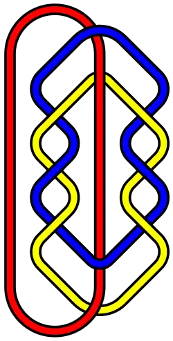
    • Barrel knot (blood knot) – joins sections of monofilament nylon line while maintaining much of the line’s inherent strength
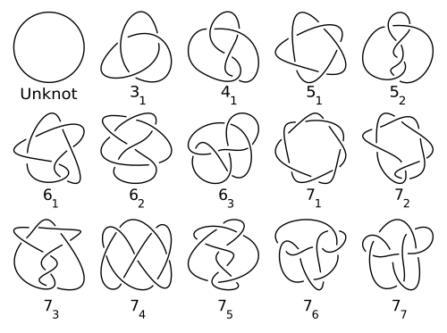
    • Basket weave knot – a family of bend and lanyard knots with a regular pattern
    • Becket hitch – any hitch made on an eye loop
    • Beer knot – bend used in tubular webbing as in slings used in rock climbing
    • Bimini twist – fishing knot used for offshore trolling and sportsfishing
    • Blackwall hitch – temporary means of attaching a rope to a hook
    • Blake’s hitch – friction hitch commonly used by arborists and tree climbers as an ascending knot
    • Blimp knot (Zeppelin bend)
    • Blood knot (barrel knot) – joins sections of monofilament nylon line while maintaining much of the line’s inherent strength
    • Blood loop knot (dropper loop) – forms a loop which is off to the side of the line
    • Boa knot – binding knot
    • Boom hitch – attach a line to a fixed object like a pipe
    • Bottle sling (jug sling) – used to create a handle for a container with a narrow tapering neck
    • Bourchier knot – a variety of heraldic knot
    • Bowen knot (heraldic knot) – not a true knot (an unknot), a continuous loop of rope laid out as an upright square shape with loops at each of the four corners
    • Bowline – forms a fixed loop at the end of a rope
    • Boling knot (archaic term for the Bowline) – forms a fixed loop at the end of a rope
    • Bowline bend
    • Bowline on a bight – makes a pair of fixed-size loops in the middle of a rope
    • Bumper knot – secures soft or loose bait in fishing
    • Bunny ears (double figure-eight loop)
    • Buntline hitch – attach a rope to an object
    • Butterfly bend – connects two ends of rope
    • Butterfly coil – a method for storing and transporting a climbing rope
    • Butterfly loop – forms a fixed loop in the middle of a rope

    C

    • Carrick bend – joins two lines of heavy rope or cable
    • Carrick bend loop – used to make a loop at the end of a rope
    • Carrick mat – flat woven decorative knot which can be used as a mat or pad
    • Cat’s paw – connects a rope to an object
    • Catshank – variant of the sheepshank, clinched by two overhand knots with the bights passed through the twists
    • Celtic button knot – a spherical decorative knot
    • Chain sinnet – method of shortening a rope or other cable
    • Chain stitch – a sewing and embroidery technique in which a series of looped stitches form a chain-like pattern
    • Chair knot (Fireman’s chair knot) – knot tied in the bight forming two adjustable, lockable loops
    • Chinese button knot – a decorative knot
    • Cleat hitch
    • Clove hitch – two successive half-hitches around an object
    • Common whipping – series of knots intended to stop a rope from unraveling
    • Constrictor knot – one of the most effective binding knots
    • Continuous ring hitching (Ringbolt hitching) – series of identical hitches made around a ring
    • Corned beef knot – binding knot often used for binding the meat of the same name while it is being cooked
    • Cow hitch – hitch knot used to attach a rope to an object
    • Cow hitch and bowline (bale sling hitch or strap hitch) – uses a continuous loop of strap to form a cow hitch around an object in order to hoist or lower it
    • Cross constrictor knot – a variant of the Constrictor knot
    • Crown knot – a knot made in the strands of the end of a rope – the start of a back splice
    • Cowboy bowline – variation of the bowline loop knot

    D

    • Diagonal lashing – lashing to bind spars or poles together to prevent racking
    • Diamond hitch – lashing technique used mainly in the field of equine packing, to secure a set of objects
    • Diamond knot (knife lanyard knot) – for forming a decorative loop on the end of a cord
    • Directional figure eight (inline figure-eight loop) – loop knot that can be made on the bight
    • Distel hitch – secure friction hitch used for rope climbing
    • Dogshank – variant of the sheepshank where the eyes formed at each end have the ends of the rope passed through
    • Donkey’s bane – variation on the diamond knot
    • Double anchorman knot – two or more pieces of rope joined together
    • Double bowline (round turn bowline) – loop knot that uses a round turn
    • Double carrick bend – join two lines together
    • Double constrictor knot – binding knot that can be difficult to untie once tightened
    • Double Englishman’s knot (double fisherman’s knot) – joins two lengths of rope
    • Double figure eight knot
    • Double figure eight bend (Flemish bend) – joins two ropes of roughly similar size
    • Double figure-eight loop – forms two parallel loops
    • Double figure eight (stevedore knot) – bulky stopper knot often tied near the end of a rope that is secure-when-slack
    • Double fisherman’s knot (grapevine knot) – joins two lengths of rope
    • Double loop (surgeon’s loop) – for making loops at the end of lines similar to the Surgeon’s knot, but with a double strand
    • Double overhand knot – extension of the regular overhand knot, made with one additional pass
    • Double overhand noose – hitch knot used to bind a rope to a carabiner
    • Double pile hitch – attaches a rope to a pole or other structure
    • Double ring knot
    • Double sheet bend – doubles a sheet bend by making an additional round turn below the first and again bringing the working end back under itself
    • Double windsor (for use in neckties) – method of tying a necktie around one’s neck and collar
    • Dropper loop – forms a loop which is off to the side of the line
    • Dutch bend, useful for tying multiple lines together
    • Dutch marine bowline (cowboy bowline) – variation of the bowline loop knot

    E

    • Egg loop a.k.a. bumper knot – secures soft or loose bait in fishing applications
    • Elusive knot
    • Englishman’s knot (fisherman’s knot) – a bend consisting of two overhand knots, each tied around the standing part of the other
    • Eskimo bowline – places a loop in the end of a rope
    • Eskimo bowstring loop knot
    • European death knot (one-sided overhand bend) – joins two ropes together
    • Eye splice – creates a permanent loop in the end of multi stranded rope by means of rope splicing

    F

    G

    • Garda hitch (alpine clutch) climbing knot that lets the rope move in only one direction
    • Girth hitch (cow hitch)
    • Good luck knot
    • Gordian knot – (mythical knot) an inextricable/complicated knot, tied by King Gordius of Phrygia, that Alexander the Great cut with a sword
    • Grantchester knot – a method of tying a necktie
    • Granny knot – secures a rope or line around an object
    • Grief knot – (what knot) combines features of granny knot and thief knot
    • Gripping sailor’s hitch – used to tie one rope to another, or a rope to a pole, when the pull is lengthwise along the object
    • Ground-line hitch – attaches a rope to an object

    H

    • Half blood knot (clinch knot) – for securing a fishing line to a fishing lure, snap or swivel
    • Half hitch – simple overhand knot, where the working end of a line is brought over and under the standing part
    • Half-Windsor knot – knot used for tying neckties
    • Halter hitch – connects a rope to an object
    • Halyard bend – a way to attach the end of a rope at right angle to a cylindrical object
    • Hammock hitch
    • Handcuff knot – tied in the bight, having two adjustable loops in opposing directions
    • Hangman’s noose (hangman’s knot) – well-known knot most often associated with its use in hanging a person
    • Harness bend – used to join two ropes together
    • Harness hitch (artillery loop) – knot with a loop on the bight for non-critical purposes
    • Heaving line knot
    • Heaving line bend – used to attach playing strings to the thick silk eyes of the anchorage knot
    • Highpoint hitch – used to attach a rope to an object
    • Highwayman’s hitch – insecure, quick-release, draw loop hitch for trivial use
    • Hitching tie – simple knot used to tie off drawstring bags that allows quick access
    • Honda knot a.k.a. lariat loop – loop knot commonly used in a lasso
    • Hoxton knot – a method of arranging a scarf about the neck
    • Hunter’s bend a.k.a. rigger’s bend – joins two lines

    I

    • Icicle hitch – excellent for connecting to a post when weight is applied to an end running parallel to the post in a specific direction
    • Improved clinch knot – used for securing a fishing line to the fishing lure
    • In-line figure-eight loop (directional figure eight) – loop knot that can be made on the bight
    • Italian hitch (Munter hitch) – simple knot commonly used by climbers and cavers as part of a life-lining or belay system

    J

    • Jack Ketch’s knot (hangman’s knot) – well-known knot most often associated with its use in hanging a person
    • Jamming knot – for constricting a bundle of objects
    • Jug sling a.k.a. bottle sling – used to create a handle for a glass or ceramic container with a slippery, narrow, tapering neck
    • Jury mast knot – for jury rigging a temporary mast on a sailboat or ship

    K

    • Karash double loop – A knot used to form leg loops as a makeshift harness
    • Killick hitch – hitch knot used to attach a rope to oddly shaped objects
    • Klemheist knot – a.k.a French Machard knot or just Machard knot. Friction hitch that grips a rope when weight is applied, and is free to move when the weight is released
    • Knot of isis – ancient Egyptian symbol of the goddess Isis; similar to a knot used to secure the garments that the Egyptian gods wore
    • Knotless knot
    • Knute hitch

    L

    • Lariat loop a.k.a. honda knot – loop knot commonly used in a lasso
    • Lark’s foot (Lark’s head, cow hitch) used to attach a rope to an object
    • Lapp knot
    • Left-hand bowline (cowboy bowline) – variation of the bowline loop knot
    • Ligature knot a.k.a. surgeon’s knot – simple modification to the reef knot that adds an extra twist when tying the first throw
    • Lighterman’s hitch (tugboat hitch) – ideal for heavy towing, or making fast to a post, bollard, or winch
    • Lineman’s loop (butterfly loop) – used to form a fixed loop in the middle of a rope
    • Lissajous knot – knot defined by parametric equations
    • Lobster buoy hitch – similar to the buntline hitch, but made with a cow hitch around the standing part rather than a clove hitch

    M

    • Machard knot – see Klemheist knot
    • Magnus hitch (rolling hitch) – used to attach a rope to a rod, pole, or other rope
    • Manharness knot (artillery loop) – knot with a loop on the bight for non-critical purposes
    • Matthew Walker knot – decorative knot that is used to keep the end of a rope from fraying
    • Marlinespike hitch – temporary knot used to attach a rod to a rope in order to form a handle
    • Marline hitching
    • Midshipman’s hitch – similar to the (taut-line hitch) – adjustable loop knot for use on lines under tension
    • Miller’s knot – binding knot used to secure the opening of a sack or bag
    • Monkey’s fist – looks somewhat like a small bunched fist/paw, most often used as the weight in a heaving line
    • Mountaineer’s coil – method used by climbers for carrying a rope
    • Munter hitch – simple knot commonly used by climbers and cavers as part of a life-lining or belay system

    N

    • Nail knot – used in fly fishing to attach the leader to the fly line
    • Nicky knot – a method of tying a necktie
    • Noose – loop at the end of a rope in which the knot slides to make the loop collapsible

    O

    P

    Q

    • Quick-release knot (Highwayman’s hitch) – insecure, quick-release, draw loop hitch for trivial use

    R

    S

    T

    • Tack knot[2]
    • Tape knot (water knot) – frequently used in climbing for joining two ends of webbing together
    • Tarbuck knot – used by climbers and was primarily used with stranded nylon rope
    • Taut-line hitch – adjustable loop knot for use on lines under tension
    • Tensionless hitch – an anchor knot used for rappelling or rope rescue.
    • Tent hitch (taut-line hitch) – adjustable loop knot for use on lines under tension
    • Thief knot – resembles the reef knot except that the free, or working, ends are on opposite sides
    • Threefoil knot – another term for a trefoil knot
    • Thumb knot a.k.a. overhand knot – one of the most fundamental knots and forms the basis of many others
    • Timber hitch – used to attach a single length of rope to a cylindrical object
    • Tom fool’s knot – good knot with which to commence a slightly fancy sheepshank
    • Transom knot – to secure two linear objects, such as spars, at right angles to each other
    • Trefoil knot – simplest example of a nontrivial knot in mathematics
    • Trident loop – fixed loop knot
    • Trilene knot – a multi purpose fishing knot
    • Triple bowline – variation of the bowline knot that is used to create three loops on one knot simultaneously
    • Triple crown knot – non-communicating double loop knot. It is secure and symmetrical, but can jam when tightened.[3]
    • Triple fisherman’s knot – a bend knot used to join two ends of rope together
    • Trucker’s hitch – used for securing loads on trucks or trailers
    • True lover’s knot – a name which has been used for many distinct knots
    • Tugboat hitch – ideal for heavy towing, or making fast to a post, bollard, or winch
    • Turle knot – used while fishing for tying a hook or fly to a leader
    • Twined Turk’s head – decorative knot with a variable number of interwoven strands forming a closed loop
    • Tumble hitch
    • Two half-hitches – an overhand knot tied around a post, followed by a half-hitch
    • Two strand overhand knot (one-sided overhand bend) – used to join two ropes together

    U

    V

    W

    • Wagoner’s hitch – compound knot commonly used for securing loads on trucks or trailers
    • Wall knot
    • Wall and crown knot – used at the end of the ropes on either side of a gangway leading onto a ship
    • Water bowline – type of knot designed for use in wet conditions where other knots may slip or jam
    • Water knot – frequently used in climbing for joining two ends of webbing together
    • Waterman’s knot – a bend with a symmetrical structure consisting of two overhand knots, each tied around the standing part of the other
    • West Country whipping – uses twine to secure the end of a rope to prevent it fraying
    • Windsor knot – a symmetrical knot used for tying a necktie around one’s neck and collar

    Y

    Z

    Sub-lists, by type

    See also

    References

    1. Philip M. Stott, Lionel G. Ripley, Michael Lavelle: The Ultimate Aberdeen Knot. In: Annals of the Royal College of Surgeons of England. 2007, volume 89, number 7, pp. 713–717 doi:10.1308/003588407X205468.
    2. “How to tie a Tack”. SelfMadeSailor. 27 October 2008. Retrieved 27 August 2023 via www.youtube.com.
    3. Ashley, Clifford W. (1944), The Ashley Book of Knots, New York: Doubleday, p. 199
    4. Ashley, Clifford W. (1944). The Ashley Book of Knots, Doubleday, p.217, #1195. ISBN 0-385-04025-3 “The Zigzag Knot is a common Stake Hitch employed in lashing wagon, sled and truck loads”
    5. Clyde Soles, Backpacker magazine’s outdoor knots: the knots you need to know, 2011, Morris Book Publishing LLC, p.101 ISBN 978-0-7627-5651-3
    6. SebringSage (24 July 2014). “Knot Tying: The Zig Zag Hitch”. Retrieved 27 August 2023 via YouTube.


    This article is adapted from “List of knots” on Wikipedia, written by its contributors, and used under CC BY-SA 4.0. Text on this page is available under the same licence. Source snapshot: Wikipedia via Kiwix, 2026-07-20.

  • List of knot theory topics


    Knot theory is the study of mathematical knots. While inspired by knots which appear in daily life in shoelaces and rope, a mathematician’s knot differs in that the ends are joined so that it cannot be undone. In precise mathematical language, a knot is an embedding of a circle in 3-dimensional Euclidean space, R3. Two mathematical knots are equivalent if one can be transformed into the other via a deformation of R3 upon itself (known as an ambient isotopy); these transformations correspond to manipulations of a knotted string that do not involve cutting the string or passing the string through itself.

    History

    Knots, links, braids

    Notation used in knot theory:

    General knot types

    Links

    General types of links:

    Tangles

    Braids

    Operations

    Elementary treatment using polygonal curves

    • elementary move (R1 move, R2 move, R3 move)
    • R-equivalent
    • delta-equivalent

    Invariants and properties

    Mathematical problems

    Theorems

    Lists


    This article is adapted from “List of knot theory topics” on Wikipedia, written by its contributors, and used under CC BY-SA 4.0. Text on this page is available under the same licence. Source snapshot: Wikipedia via Kiwix, 2026-07-20.