The Borromean rings, a link with three components each equivalent to the unknot.
In mathematical knot theory, a link is a collection of knots that do not intersect, but which may be linked (or knotted) together. A knot can be described as a link with one component. Links and knots are studied in a branch of mathematics called knot theory. Implicit in this definition is that there is a trivial reference link, usually called the unlink, but the word is also sometimes used in context where there is no notion of a trivial link.
A Hopf link spanned by a twisted annulus.
For example, a co-dimension 2 link in 3-dimensional space is a subspace of 3-dimensional Euclidean space (or often the 3-sphere) whose connected components are homeomorphic to circles.
The simplest nontrivial example of a link with more than one component is called the Hopf link, which consists of two circles (or unknots) linked together once. The circles in
the Borromean rings are collectively linked despite the fact that no two of them are directly linked. The Borromean rings thus form a Brunnian link and in fact constitute the simplest such link.
The notion of a link can be generalized in a number of ways.
General manifolds
Frequently the word link is used to describe any submanifold of the sphere diffeomorphic to a disjoint union of a finite number of spheres, .
In full generality, the word link is essentially the same as the word knot – the context is that one has a submanifold M of a manifold N (considered to be trivially embedded) and a non-trivial embedding of M in N, non-trivial in the sense that the 2nd embedding is not isotopic to the 1st. If M is disconnected, the embedding is called a link (or said to be linked). If M is connected, it is called a knot.
Tangles, string links, and braids
While (1-dimensional) links are defined as embeddings of circles, it is often interesting and especially technically useful to consider embedded intervals (strands), as in braid theory.
Most generally, one can consider a tangle[1][2] – a tangle is an embedding
of a (smooth) compact 1-manifold with boundary into the plane times the interval such that the boundary is embedded in
().
The type of a tangle is the manifold X, together with a fixed embedding of
Concretely, a connected compact 1-manifold with boundary is an interval or a circle (compactness rules out the open interval and the half-open interval neither of which yields non-trivial embeddings since the open end means that they can be shrunk to a point), so a possibly disconnected compact 1-manifold is a collection of n intervals and m circles The condition that the boundary of X lies in
says that intervals either connect two lines or connect two points on one of the lines, but imposes no conditions on the circles.
One may view tangles as having a vertical direction (I), lying between and possibly connecting two lines
( and ),
and then being able to move in a two-dimensional horizontal direction ()
between these lines; one can project these to form a tangle diagram, analogous to a knot diagram.
Tangles include links (if X consists of circles only), braids, and others besides – for example, a strand connecting the two lines together with a circle linked around it.
In this context, a braid is defined as a tangle which is always going down – whose derivative always has a non-zero component in the vertical (I) direction. In particular, it must consist solely of intervals, and not double back on itself; however, no specification is made on where on the line the ends lie.
A string link is a tangle consisting of only intervals, with the ends of each strand required to lie at (0,0),(0,1),(1,0),(1,1),(2,0),(2,1),… – i.e., connecting the integers, and ending in the same order that they began (one may use any other fixed set of points); if this has ℓ components, we call it an “ℓ-component string link”. A string link need not be a braid – it may double back on itself, such as a two-component string link that features an overhand knot. A braid that is also a string link is called a pure braid, and corresponds with the usual such notion.
The key technical value of tangles and string links is that they have algebraic structure. Isotopy classes of tangles form a tensor category, where for the category structure, one can compose two tangles if the bottom end of one equals the top end of the other (so the boundaries can be stitched together), by stacking them – they do not literally form a category (pointwise) because there is no identity, since even a trivial tangle takes up vertical space, but up to isotopy they do. The tensor structure is given by juxtaposition of tangles – putting one tangle to the right of the other.
For a fixed ℓ, isotopy classes of ℓ-component string links form a monoid (one can compose all ℓ-component string links, and there is an identity), but not a group, as isotopy classes of string links need not have inverses. However, concordance classes (and thus also homotopy classes) of string links do have inverses, where inverse is given by flipping the string link upside down, and thus form a group.
Every link can be cut apart to form a string link, though this is not unique, and invariants of links can sometimes be understood as invariants of string links – this is the case for Milnor’s invariants, for instance. Compare with closed braids.
↑Habegger, Nathan; Lin, X.S. (1990), “The classification of links up to homotopy”, Journal of the American Mathematical Society, 2, 3 (2), American Mathematical Society: 389–419, doi:10.2307/1990959, JSTOR1990959
↑Habegger, Nathan; Masbaum, Gregor (2000), “The Kontsevich integral and Milnor’s invariants”, Topology, 39 (6): 1253–1289, CiteSeerX10.1.1.31.6675, doi:10.1016/S0040-9383(99)00041-5
This article is adapted from “Link (knot theory)” on Wikipedia, written by its contributors, and used under CC BY-SA 4.0. Text on this page is available under the same licence. Source snapshot: Wikipedia via Kiwix, 2026-07-20.
The standard contact structure on R3. Each point in R3 has a plane associated to it by the contact structure, in this case as the kernel of the one-form dz − y dx.
In mathematics, a Legendrian knot often refers to a smooth embedding of the circle into , which is tangent to the standard contact structure on . It is the lowest-dimensional case of a Legendrian submanifold, which is an embedding of a k-dimensional manifold into a (2k+1)-dimensional contact manifold that is always tangent to the contact hyperplane.
Classification
Two smooth knots are equivalent if there is a way to smoothly deform one into the other. That is, if there is a smooth ambient isotopy from one to the other.
Similarly, two Legendrian knots are equivalent if there is a way to smoothly deform one into the other, such that any intermediate knot is still a Legendrian knot. Two equivalent Legendrian knots are equivalent as smooth knots, but the converse is false.
Many inequivalent Legendrian knots can be distinguished by considering their Thurston-Bennequin invariants and rotation number, which are together known as the “classical invariants” of Legendrian knots. More sophisticated invariants have been constructed, including one constructed combinatorially by Chekanov and using holomorphic discs by Eliashberg. This Chekanov-Eliashberg invariant yields an invariant for loops of Legendrian knots by considering the monodromy of the loops. This has yielded noncontractible loops of Legendrian knots which are contractible in the space of all knots.
Any Legendrian knot may be perturbed to a transverse knot (a knot transverse to a contact structure) by pushing off in a direction transverse to the contact planes. The set of isomorphism classes of Legendrian knots modulo negative Legendrian stabilizations is in bijection with the set of transverse knots.
This article is adapted from “Legendrian knot” on Wikipedia, written by its contributors, and used under CC BY-SA 4.0. Text on this page is available under the same licence. Source snapshot: Wikipedia via Kiwix, 2026-07-20.
Bamboo scaffolding secured with lashings in Kowloon.
A lashing is an arrangement of rope, wire, or webbing with linking device used to secure and fasten two or more items together in a somewhat rigid manner. Lashings are most commonly applied to timber poles, and are commonly associated with cargo, containerization, the Scouting movement, sailors, and gardeners.
In its most basic sense, lashing is about attaching two poles (or spars) together. It consists of “wraps”, winding the rope around the poles, and “fraps”, winding the around between the poles and around the wraps to tighten them.[1]
It has been imagined that the first lashing made by humans was wrapping a few strips of bark around a stone to hold it to a tree branch to make an ax to hunt and build with. In modern times, the same methods are used, but strips of bark and vines have been replaced with natural and synthetic fiber ropes. Scouts and campers use lashings to build camp gadgets and improve their campsites for comfort and convenience, including the building of rafts for transport and competitive events. Lashings are also used in pioneering, the art of creating structures such as bridges and towers, using ropes and wooden spars.
There are still areas in the world where lashing spars (or poles) is the basic means of building.
Types
A square lashing binding a wooden spar to a tree trunk. The rope turns between the tree and spar are the frapping.
Square lashing
Square Lashing
Square lashing is a type of lashing used to bind spars together, at right angles to one another. There are different types, but all consist of a series of wraps around the spars, and frapping around the line running between the spars.[1]
Diagonal lashing
Diagonal lashing is a type of lashing used to bind spars or poles together, to prevent racking. It gets its name from the fact that the wrapping turns cross the poles diagonally and is used to spring poles together where they do not touch as in the X-brace of a trestle.[1][2]
Shear lashing
Shear lashing (two-spar shear lashing) also spelled “sheer lashing” is used for lashing together two parallel spars which will be opened out of the parallel to form sheer legs as in the formation of an A-frame. The clove hitch is tied around one leg only and frapping turns are taken between the poles.[1][3]
Round lashing
The round lashing is most frequently used to join two poles together to extend their length. Typically, two lashings are used a reasonable distance apart for extra strength. In the simple version, a clove hitch is tied around both poles and there are no frapping turns.[1][4]
The nautical term gammon means a round lashing of rope or iron hardware to attach a mast to a boat or ship.[5]
Tripod lashing
The tripod lashing is used to join three spars together to form a self supporting structure. Two structures can be used to support a crossbar or platform.[1] Other names are gyn lashing, figure of eight lashing, and three-spar shear lashing. If the lashing is tied around three spars, then the structure is called a tripod, but quadpods can also be made by using four spars.
This article is adapted from “Lashing (ropework)” on Wikipedia, written by its contributors, and used under CC BY-SA 4.0. Text on this page is available under the same licence. Source snapshot: Wikipedia via Kiwix, 2026-07-20.
A lanyard is a length of cord, webbing, or strap that may serve any of various functions, which include a means of attachment, restraint, retrieval, activation, and deactivation.
Origins
The earliest references to lanyards date from 15th century France: “lanière” was a thong or strap-on apparatus.[1]
A typical marlinspike with lanyard
Bosun’s pipe, marlinspike, and small knives typically had a lanyard consisting of a string loop tied together with a diamond knot. It helped secure the item and gave an extended grip over a small handle.
In the French military, lanyards were used to connect a pistol, sword, or whistle (for signaling) to a uniform semi-permanently. Lanyards were used by mounted cavalry on land and naval officers at sea. A pistol lanyard can be easily removed and reattached by the user, but will stay connected to the pistol whether it is drawn for use or it is placed into a holster for carrying.
In the military, lanyards of various colour combinations and braid patterns are worn on the shoulders of uniforms to denote the wearer’s qualification or regimental affiliation.[2] In horse regiments, lanyards were worn on the left, enabling a rider to pull a whistle from the left tunic pocket and maintain communication with his troop. Members of the British Royal Artillery wear a lanyard which originally held a key for adjusting the fuzes of explosive shells.[3]
Functions
An attachment lanyard is a light duty tether worn around the neck, shoulder, wrist or attached to the belt as a sling to conveniently carry items such as keys or identification cards,[4] or as a safety harness to prevent accidental dropping of valuable handheld items such as a camera.
A restraint lanyard is a safety lanyard used by construction workers, such as a lineman.
A retrieval lanyard is a nylon webbing lanyard used to raise and lower workers into confined spaces, such as storage tanks.
An activation lanyard is a lanyard used to fire an artillery piece or arm the fuze on a bomb leaving an aircraft.[5]
A deactivation lanyard is a dead man’s switch, where pulling a lanyard free will disable a dangerous device.
Styles and materials
Light-duty webbing lanyard for attaching keys, with a metal clip similar to that of a leash
The style, design or material used will vary depending on end-purpose of the lanyard. Lanyard materials include polyester, nylon, satin, silk, polyethylene terephthalate (PET), braided leather or braided paracord.
Common styles
Polyester imprinted lanyards
Nylon imprinted lanyards
Tube imprinted lanyards
Dye-sublimated lanyards or full-color lanyards
Accessory for electronics
A USB flash drive with a webbing lanyard that includes a safety break-away feature – a predetermined and in this case reattachable segment (in black) meant to prevent accidental strangulation when the lanyard is worn around the neck
Lanyards are widely used with small electronic devices such as cameras, MP3 players and USB flash drives to prevent loss or dropping. Electronics designed to take a lanyard usually have a small through-hole built into a corner or edge of the case or anchored to the frame of the device; the corresponding lanyard generally has a loop of thread on the end that is attached to that hole with a simple knot, usually a cow hitch. Some earphones incorporate the audio signal into the lanyard, meaning it doubles up as headphone cords as well. The Wii Remote wrist strap is a form of lanyard, keeping the device attached to a player’s arm during the often vigorous movements involved in its use.
Badge or identification holder
Lanyards are commonly used to display badges, tickets or ID cards for identification where security is required, such as businesses, corporations, hospitals, prisons, conventions, trade fairs, and backstage passes used in the entertainment industry. Such lanyards are often made of braided or woven fabric or split with a clip attached to the end. A plastic pouch or badge holder with at least one clear side is attached to the lanyard with the person’s name badge or ID card. Occasionally, small items like business cards, pens or tools can be placed behind the badge for easy access. Lanyards can also be used as keychains, particularly in situations where keys can easily be lost, such as gyms, public pools and communal showers.
In these cases, lanyards may be customised with the related name and/or logo of the event, business, or organisation. Lanyards can feature a variety of customisation techniques including screen-printing, Jacquard loom weaving, heat transfer, and offset printing.
Safety strap
Lanyards are also often attached to dead man’s switches or “kill switches” on dangerous machinery, such as large industrial cutting or slicing machines, vehicles, jet-skis or trains, and exercise treadmills, so that if the operator suddenly becomes incapacitated, their fall will pull on the lanyard attached to their wrist, which will then pull the switch to immediately stop the machine or vehicle.
Some law enforcement officers and members of the military utilise specialised lanyards to keep sidearms from falling to the ground during missions.
Many ID card lanyards have a built-in feature known as a “breakaway” closure. Breakaway lanyards release when pulled or when pressure is applied. This prevents choking or hanging. Lanyards with a breakaway feature are most often used in hospitals and healthcare clinics, schools, nursing homes, child care facilities, and factories that require employees to operate machinery.
Lineman lanyards
Lineman lanyards are used by lineworker utility and other workers to prevent falls, although similar straps are also used recreationally by mountain climbers. This type of lanyard will have a section of heavy-duty nylon strapping attached to a metal ring or carabiner which tightens around an attachment point. The strap may be a fixed length or adjustable, and will attach to the wearer to support them against a fixed object or pole.
A white lanyard has formed part of the uniform of Britain’s Royal Artillery (RA) since the end of the 19th century. Originally a simple cord carrying a fuse key, the braided and whitened lanyard became the recognised distinction of a Gunner.[6] The distinction was extended to women of the Auxiliary Territorial Service attached to RA units during World War II.[7] Certain battalions descended from the Durham Light Infantry wore green lanyards to denote their past links with the regiment, whose uniform had a dark green facing colour from 1903 onwards.[8][9]
Royal Naval ratings wear a white lanyard when dressed in No. 1 uniform; the origin of the lanyard was to carry a pouch of gunpowder for the cannon.
See also
Access badge
Halyard
Rope splicing
References
↑Wedgwood, Hensleigh (1855). “On False Etymologies”. Transactions of the Philological Society (6): 68.
↑“lanyard.” The Macquarie Dictionary. South Yarra: The Macquarie Library Pty Ltd., 2005. Credo Reference. Web. 1 October 2012.
↑Col J.D. Sainsbury, The Hertfordshire Yeomanry Regiments, Royal Artillery, Part 2: The Heavy Anti-Aircraft Regiment 1938–1945 and the Searchlight Battery 1937–1945; Part 3: The Post-war Units 1947–2002, Welwyn: Hertfordshire Yeomanry and Artillery Trust/Hart Books, 2003, ISBN0-948527-06-4, Plate 9, p. 7.
↑Norman E.H. Litchfield, The Territorial Artillery 1908–1988 (Their Lineage, Uniforms and Badges), Nottingham: Sherwood Press, 1992, ISBN0-9508205-2-0, pp. 56–8.
↑Ward, S G P 1962 Faithful. The Story of the Durham Light Infantry Naval and Military Press ISBN9781845741471, p. 461.
This article is adapted from “Lanyard” on Wikipedia, written by its contributors, and used under CC BY-SA 4.0. Text on this page is available under the same licence. Source snapshot: Wikipedia via Kiwix, 2026-07-20.
Kumihimo (組み紐) is a traditional Japanese artform and craftwork for making braids and cords.[1][2] In the past, kumihimo decorations were used as accessories for kimono as well as samurai armor.[3]Japanese braiding, as kumihimo is sometimes known in English, is also associated with Shinto rituals and religious services.[2] Literally meaning “gathered threads”, kumihimo are made by interlacing reels of yarn, commonly silk, with the use of traditional, specialised looms – either a marudai (丸台, lit.‘round stand‘)[2] or a takadai (高台) (also known as a kōdai).
There are a number of different styles of kumihimo weaving, which variously create a braided cord ranging from very flat to almost entirely rounded.[1]Kumihimo cords are used as obijime, cords worn belted around the front of some obi when wearing kimono.
History
Sageo cord for tachi (Japanese long sword) made of kumihimo, with Tokugawa clan mon, Edo periodŌ-yoroi decorated with kumihimo owned by Shimazu Nariakira
During the Jomon period, primitive braids appeared that could be considered the predecessors of kumihimo, or Japan’s first kumihimo. During this period, braids were used to create patterns on Jomon pottery, and the indentations of the braids attached to the clay became the decoration of the pottery.[4][5][6]
Kumihimo, which falls into the category of crafts, was introduced to Japan from China via the Korean peninsula around 700 AD.[7][8] When the art first arrived in Japan, it was used to decorate Buddhist scrolls and other votive items. The city of Nara emerged as a centre of cultural and artistic exchange and became the point of introductory of kumihimo to Japan.[9]
When regular trade and cultural exchange with China ceased Heian period (794-1185), kumihimo culture flourished, combining several earlier techniques to create a uniquely Japanese design that was more complex than before. From the mid-Heian period, kumihimo was also used to decorate ō-yoroi, the Japanese armour worn by samurai. In addition to functionality, the aesthetics of the ō-yoroi were considered important, and sometimes 300 meters of kumihimo were used for each piece of armor. Kumihimo was also used to tie tachi (Japanese long sword) and harnesses around the waist. From the late Heian period, nioi-odoshi (匂威) and susogo (裾濃), a weaving technique characterized by gradations of color, appeared.[4][5][6][10]
During the Kamakura period (1185-1333), various new weaving techniques for kumihimo appeared. Kikko-gumi (亀甲組), which imitates the pattern of a turtle shell, appeared for the first time in this period and was used as kumihimo for armor.[5][10]
During the Muromachi period (1333-1573), kumihimo was used as a decorative weave for teaware used in the Japanese tea ceremony. Taking advantage of the wabi-sabi aesthetic that emerged during this period, this weaving method became popular for designs that were more subdued yet prestigious than the more traditional and flamboyant designs. During this period, dan-odoshi (段威), a weaving technique using different colors in a striped pattern, appeared.[4][5][6]
During the Azuchi-Momoyama period (1568-1600), a weaving technique called mongara-odoshi (紋柄威), in which mon (family emblem) and designs were expressed in two colors, appeared.[6]
Three tachi decorated with kumihimo (sageo cords), Edo period
During the Edo period (1603-1867), with the advent of a more peaceful society, the aesthetic value of Japanese swords became increasingly important. As the demand for kumihimo for Japanese swords increased, frames called takadai and naikidai were invented to make kumihimo, and the technique of braiding developed dramatically, giving rise to many new techniques. Kumihimo spread to the general public chōnin class and was used as braids and cords for attaching haori (traditional Japanese jacket), inro (traditional Japanese portable case), and netsuke. During this period, geisha began to use the otaiko-musubi (御太鼓結び) knot to tie obi (kimono belt), which spread to the general public and dramatically increased the decorative value of the obi. As a result, decorative kumihimo were used as obijime to support the obi. The technique of ayadashi (綾出), which produces patterns and characters on the kumihimo, appeared during this period, and various new methods of weaving patterns appeared along with the popularity of the iki aesthetic.[4][5][6][10]
A vermilion obijime tied over the kimono and obi
During the Meiji era (1868-1912), the demand for kumihimo to decorate Japanese swords decreased drastically due to the Sword Abolishment Edict and the disappearance of the samurai class. After that, kumihimo survived mainly as obijime to support obi.[4][5][6][10]
Kumihimo braids were first created by using fingerloop braiding to weave different yarns together. Later, tools such as the marudai and the takadai were developed, allowing more complex braids to be woven in a shorter amount of time.
Modern kumihimo: 20th and 21st centuries
Japanese braiding is being used in other areas in addition to its traditional uses, and has been taken up by arts and craft communities outside of Japan.[11][12]Kumihimo has gained in popularity outside of Japan, with an increasing number of beginner books available in languages other than Japanese.[13][14][15][16][17] There is also a Journal of the American Kumihimo Society.[12]
In contrast to the interest in Japanese braiding as a craft for all, the city of Columbus, Georgia, USA, commissioned Junichi Arai (1932–2017) to create a permanent 12 × 9 metre metallic fibre artwork consisting of 200 stainless steel kumihimo braidings that produced kinetic waves.[11] Arai is considered an important innovator who raised textiles from craft to art. Akiko Moriyama describes him thus: “Arai embodies everything about Japanese textiles, from the challenges to the possibilities.”[11] Arai’s installation opened at for the River Center for Performing Arts in 2003.[11]
In the present day, modern variations of kumihimo weaving discs exist, typically made of firm, dense foam with (typically) 32 notches around the edge, creating the tension necessary for weaving kumihimo. These discs are considered to be a more affordable and portable alternative to a traditional marudai, with many different sizes and shapes of disc available for purchase.
However, a modern foam kumihimo disc is considered less versatile than a traditional marudai. A traditional marudai allows the weaver to use as many yarns of as many thicknesses as desired, and to create braids which are flat, four sided, or hollow. A foam kumihimo disc constrains the weaver to no more than 32 yarns that must not be thicker than the notch allows, and does not enable the creation of flat braids. To make a flat braid a separate rectangular or square “disc” must be made or purchased.
Types
The three prominent types of kumihimo are kado-uchi himo (角打ち紐), hira-uchi himo (平打紐), and maru-uchi himo (丸打紐).[7]
Tama bobbins
Related terms
A marudai stand featuring a partially finished kumihimo, weighted with a tama (lit.‘ball‘) weight to keep tension whilst weaving
Kagami – the top braiding surface on a marudai; Japanese for “mirror”.
Kongō Gumi – a class of patterns for round cord all involving eight threads folded in half for a total of sixteen strands. In clockwise order, each bobbin is moved to the opposite side. When different combinations of thread color are used, many interesting patterns emerge, including diagonal stripes, diamonds on a background, triangles resembling hearts, and tiny six-petalled flowers.
Marudai or maru dai – the frame for the braiding; maru dai Japanese for “round stand”.
Mizuhiki, decorative cords used to decorate objects such as shūgi-bukuro envelopes.
Obijime – the broad cloth sash used in traditional dress; a kumihimo belt, called the obijime, is tied around the obi.
Takadai – a takadai is a large, rectangular frame for creating flat, oblique kumihimo braids.
Tama – bobbins. The thread is kept from unwinding by passing the thread under itself, forming a loop around the tama. True silk is a hollow fiber with a rough surface that resists slipping past the loop unless gently pulled. For synthetic fibers, a flexible plastic “clamshell” bobbin may be preferable.
12Kinoshita, Masako (1986). “A Braiding Technique Documented in an Early Nineteenth-Century Japanese Treatise” Soshun Bik‾”“. Textile Museum Journal. 25: 47–65 – via EBSCOhost Art & Architecture Source.
123Kimura, Akiko; Tada, Makiko; Uozumi, Tadashi; Goto, Akihiko (2018), “Teaching Method of Technique to Make the Braiding”, in Trzcielinski, Stefan (ed.), Advances in Ergonomics of Manufacturing: Managing the Enterprise of the Future, vol.606, Cham: Springer International Publishing, pp.310–321, doi:10.1007/978-3-319-60474-9_29, ISBN978-3-319-60473-2, retrieved 2024-07-09
1234組紐の歴史 (in Japanese). Yushiki kumihimo domyo. Archived from the original on 13 February 2025. Retrieved 13 February 2025.
1234Moriyama, Akiko (2020). Harris, Jennifer (ed.). Japanese Textile Culture in A Companion to Textile Culture. Wiley-Blackwell companions to art history. Hoboken, NJ: John Wiley & Sons, Inc. pp.353–370. ISBN978-1-118-76860-0.
12Hardy, Beth; Benner, Carol; Haushalter-Oliver, Carolyn; Mutter, Debbie; Shirashi, Diana; Imperia, Giovanna; Pigot, Jan; Peterson, Jane; Johansen, Katia; Tada, Makiko; Jeppesen, Margaret; Tada, Masumi; Nielson, Rosalie; Berlin, Shirley; Guang, Yin (2020). Gaskell, Adrienne; Buenger, Katherine (eds.). “Gathering Threads”. Journal of the North American Kumihimo Society.
This article is adapted from “Kumihimo” on Wikipedia, written by its contributors, and used under CC BY-SA 4.0. Text on this page is available under the same licence. Source snapshot: Wikipedia via Kiwix, 2026-07-20.
Koroba is a type of Yoruba braid hairstyle.[1] Koroba means basket in the Yoruba language. The name comes from the shape and design of the hairstyle.[2] It is shaped like a basket upside down. The braids come from the middle of the head, downwards and spread to other parts of the head. It is a rounded circular hairstyle that comes straight or curled at the ends. Koroba is one of the indigenous Yoruba braids and represents one of the many traditional African braids.[3][4][5]
This article is adapted from “Koroba (hairstyle)” on Wikipedia, written by its contributors, and used under CC BY-SA 4.0. Text on this page is available under the same licence. Source snapshot: Wikipedia via Kiwix, 2026-07-20.
In the mathematical theory of knots, the Kontsevich invariant, also known as the Kontsevich integral[1] of an oriented framed link, is a universal Vassiliev invariant[2] in the sense that any coefficient of the Kontsevich invariant is of a finite type, and conversely any finite type invariant can be presented as a linear combination of such coefficients. It was defined by Maxim Kontsevich.
The Kontsevich invariant is a universal quantum invariant in the sense that any quantum invariant may be recovered by substituting the appropriate weight system into any Jacobi diagram.
Definition
The Kontsevich invariant is defined by monodromy along solutions of the Knizhnik–Zamolodchikov equations.
Jacobi diagram and Chord diagram
Definition
an example of a Jacobi diagram
Let X be a circle (which is a 1-dimensional manifold). As is shown in the figure on the right, a Jacobi diagram with order n is the graph with 2n vertices, with the external circle depicted as solid line circle and with dashed lines called inner graph, which satisfies the following conditions:
The orientation is given only to the external circle.
The vertices have values 1 or 3. The valued 3 vertices are connected to one of the other edge with clockwise or anti-clockwise direction depicted as the little directed circle. The valued 1 vertices are connected to the external circle without multiplicity, ordered by the orientation of the circle.
The edges on G are called chords. We denote as A(X) the quotient space of the commutative group generated by all the Jacobi diagrams on X divided by the following relations:
(The AS relation) + = 0
(The IHX relation) = −
(The STU relation) = −
(The FI relation) = 0.
A diagram without vertices valued 3 is called a chord diagram or Gauss diagram. If every connected component of a graph G has a vertex valued 3, then we can make the Jacobi diagram into a Chord diagram using the STU relation recursively. If we restrict ourselves only to chord diagrams, then the above four relations are reduced to the following two relations:
(The four term relation) − + − = 0.
(The FI relation) = 0.
Properties
The degree of a Jacobi diagram is defined to be the half of the sum of the number of its vertices with value 1 and one with value 3. It is the number of chords in the Chord diagram transformed from the Jacobi diagram.
Just like for the tangles, the Jacobi diagrams form a monoidal category with the composition as the compiling of Jacobi diagrams along up and down direction and the tensor product as juxtapositioning Jacobi diagrams.
In the special case where X is an interval I, A(X) will be a commutative algebra. Viewing A(S1) as the algebra with multiplication as connected sums, A(S1) is isomorphic to A(I).
A Jacobi diagram can be viewed as abstraction of representations of the tensor algebra generated by Lie algebras, which allows us to define some operations analogous to coproducts, counits and antipodes of Hopf algebras.
Since the Vassiliev invariants (or finite type invariants) are closely related to chord diagrams, one can construct a singular knot from a chord diagram G on S1. Kn denoting the space generated by all the singular knots with degree n, every such G determines a unique element in Km / Km+1.
Weight system
A map from the Jacobi diagrams to the positive integers is called a weight system. The map extended to the space A(X) is also called the weight system. They have the following properties:
Let g be a semisimple Lie algebra and ρ its representation. We obtain a weight system by “substituting” the invariant tensor of g into the chord of a Jacobi diagram and ρ into the underlying manifold X of the Jacobi diagram.
We can view the vertices with value 3 of the Jacobi diagram as the bracket product of the Lie algebra, solid line arrows as the representation space of ρ, and the vertices with value 1 as the action of the Lie algebra.
The IHX relation and the STU relation correspond respectively to the Jacobi identity and the definition of the representation
Jacobi diagrams were introduced as analogues of Feynman diagrams when Kontsevich defined knot invariants by iterated integrals in the first half of 1990s.[2] He represented singular points of singular knots by chords, i.e. he treated only with chord diagrams. D. Bar-Natan later formulated them as the 1-3 valued graphs and studied their algebraic properties, and called them “Chinese character diagrams” in his paper.[4] Several terms such as chord diagrams, web diagrams, or Feynman diagrams were used to refer them, but they have been called Jacobi diagrams since around 2000, because the IHX relation corresponds to the Jacobi identity for Lie algebras.
We can interpret them from a more general point of view by claspers, which were defined independently by Goussarov and Kazuo Habiro in the later half of the 1990s.
References
↑Chmutov, Sergei; Duzhi, Sergei (2012). Weisstein, Eric W (ed.). “Kontsevich Integral”. Mathworld. Wolfram Web Resource. Retrieved 4 December 2012.
Ohtsuki, Tomotada (2001). Quantum Invariants – A Study of Knots, 3-Manifolds, and their Sets (1sted.). World Scientific Publishing Company. ISBN9789810246754. OL9195378M.
This article is adapted from “Kontsevich invariant” on Wikipedia, written by its contributors, and used under CC BY-SA 4.0. Text on this page is available under the same licence. Source snapshot: Wikipedia via Kiwix, 2026-07-20.
Vases in Pekin stitch, Qing dynasty (1644–1912), China
A knotted stitch, also known as knot stitch, is any embroidery technique in which the yarn or thread is knotted around itself. A knotted stitch is a type of decorative embroidery stitches which form three-dimensional knots on the surface of a textile.[1] Common knotted stitches include French knots, coral stitch,[2][3] and Pekin knot (also known as forbidden stitch, Pekin stitch, and seed stitch)[4][5] which is sometimes also referred as French knot although there is a difference in techniques between these two stitches.[1] Knotted stitches can be subdivided into individual or detached knots, continuous knotted stitches, and knotted edgings.
History
Knotted embroidery originated in ancient China; the oldest example of it dates from the Warring States period in the form a pair of silk shoes.[1] Knotted embroidery was popular in the Han dynasty and fine silk clothing were embellished with the Pekin knot in this period.[1] Knotted embroidery were also used on the mandarin square of the Ming and Qing court clothing of officials.[1] The Pekin knot is one of the two main types of Chinese embroidery stitches, with the other being the satin stitch.[5]
Embroideries tradition which started in China were passed to other countries through the Silk Road.[6]
Roundels in Peking knot and satin stitch, Qing dynasty.Contemporary design of French knots surrounded by chain stitch from a sampler in the form of a challah cover.
Embroideries from China and Western Asia were imported to the British Isles, North America and Western Europe by the British East India Company in the 1690s along with many other traded goods.[1] Eastern knotted embroidery became popular among Westerners.[1] The liking for the Pekin knot eventually influenced the development of tatting in Western Europe and the British Isles when Europeans sought the knotted effects of the stitches but did not want the time-consuming process of stitching tightly packed little knots continuously for long hours.[1]
Applications
Individual knots are often found used as detached filling stitches.[3]
Knotted edgings are used as a decorative trims, and can also be used to fill open spaces in cutwork and in needlelace.
Caulfield, S.F.A., and B.C. Saward, The Dictionary of Needlework, 1885.
Christie, Mrs. Archibald (Grace Christie), Embroidery and Tapestry Weaving, London, John Hogg, 1912, online at Project Gutenberg
Christie, Mrs. Archibald (Grace Christie), Samplers and Stitches, a handbook of the embroiderer’s art, London 1920
Enthoven, Jacqueline: The Creative Stitches of Embroidery, Van Norstrand Rheinhold, 1964, ISBN0-442-22318-8
Reader’s Digest, Complete Guide to Needlework. The Reader’s Digest Association, Inc. (March 1992). ISBN0-89577-059-8
This article is adapted from “Knotted stitch” on Wikipedia, written by its contributors, and used under CC BY-SA 4.0. Text on this page is available under the same licence. Source snapshot: Wikipedia via Kiwix, 2026-07-20.
Examples of different knots including the unknot (top left) and the trefoil knot (below it)A knot diagram of the trefoil knot, the simplest non-trivial knot
In topology, knot theory is the study of mathematical knots. While inspired by knots which appear in daily life, such as those in shoelaces and rope, a mathematical knot differs in that the ends are joined so it cannot be undone, the simplest knot being a ring (or “unknot“). In mathematical language, a knot is an embedding of a circle in 3-dimensional Euclidean space, . Two mathematical knots are equivalent if one can be transformed into the other via a deformation of upon itself (known as an ambient isotopy); these transformations correspond to manipulations of a knotted string that do not involve cutting it or passing it through itself.
Knots can be described in various ways. Using different description methods, there may be more than one description of the same knot. For example, a common method of describing a knot is a planar diagram called a knot diagram, in which any knot can be drawn in many different ways. Therefore, a fundamental problem in knot theory is determining when two descriptions represent the same knot.
A complete algorithmic solution to this problem exists, which has unknown complexity.[1] In practice, knots are often distinguished using a knot invariant, a “quantity” which is the same when computed from different descriptions of a knot. Important invariants include knot polynomials, knot groups, and hyperbolic invariants.
The original motivation for the founders of knot theory was to create a table of knots and links, which are knots of several components entangled with each other. More than six billion knots and links have been tabulated since the beginnings of knot theory in the 19th century.
To gain further insight, mathematicians have generalized the knot concept in several ways. Knots can be considered in other three-dimensional spaces and objects other than circles can be used; see knot (mathematics). For example, a higher-dimensional knot is an n-dimensional sphere embedded in (n+2)-dimensional Euclidean space. Knot theory can also be extended to describe entanglement in open curves, which is used to study knots in proteins, DNA, and physical ropes.
History
Intricate Celtic knotwork in the 1200-year-old Book of Kells
Archaeologists have discovered that knot tying dates back to prehistoric times. Besides their uses such as recording information and tying objects together, knots have interested humans for their aesthetics and spiritual symbolism. Knots appear in various forms of Chinese artwork dating from several centuries BC (see Chinese knotting). The endless knot appears in Tibetan Buddhism, while the Borromean rings have made repeated appearances in different cultures, often representing strength in unity. The Celtic monks who created the Book of Kells lavished entire pages with intricate Celtic knotwork.
The first knot tabulator, Peter Guthrie Tait
A mathematical theory of knots was first developed in 1771 by Alexandre-Théophile Vandermonde who explicitly noted the importance of topological features when discussing the properties of knots related to the geometry of position. Mathematical studies of knots began in the 19th century with Carl Friedrich Gauss, who defined the linking integral(Silver 2006). In the 1860s, Lord Kelvin’s theory that atoms were knots in the aether led to Peter Guthrie Tait’s creation of the first knot tables for complete classification. Tait, in 1885, published a table of knots with up to ten crossings, and what came to be known as the Tait conjectures. This record motivated the early knot theorists, but knot theory eventually became part of the emerging subject of topology.
These topologists in the early part of the 20th century—Max Dehn, J. W. Alexander, and others—studied knots from the point of view of the knot group and invariants from homology theory such as the Alexander polynomial. This would be the main approach to knot theory until a series of breakthroughs transformed the subject.
In the late 1970s, William Thurston introduced hyperbolic geometry into the study of knots with the hyperbolization theorem. Many knots were shown to be hyperbolic knots, enabling the use of geometry in defining new, powerful knot invariants. The discovery of the Jones polynomial by Vaughan Jones in 1984 (Sossinsky 2002, pp.71–89), and subsequent contributions from Edward Witten, Maxim Kontsevich, Louis Kauffman, and others, revealed deep connections between knot theory and mathematical methods in statistical mechanics and quantum field theory. A plethora of knot invariants have been invented since then, utilizing sophisticated tools such as quantum groups and Floer homology.
In the last several decades of the 20th century, scientists became interested in studying physical knots in order to understand knotting phenomena in DNA and other polymers. Knot theory can be used to determine if a molecule is chiral (has a “handedness”) or not (Simon 1986). Tangles, strings with both ends fixed in place, have been effectively used in studying the action of topoisomerase on DNA (Flapan 2000). Knot theory may be crucial in the construction of quantum computers, through the model of topological quantum computation (Collins 2006).
Knot equivalence
On the left, the unknot, and a knot equivalent to it. It can be more difficult to determine whether complex knots, such as the one on the right, are equivalent to the unknot.
A knot is created by beginning with a one-dimensional line segment, wrapping it around itself arbitrarily, and then fusing its two free ends together to form a closed loop (Adams 2004)(Sossinsky 2002). Simply, we can say a knot is a “simple closed curve” (see Curve) — that is: a “nearly” injective and continuous function , with the only “non-injectivity” being . Topologists consider knots and other entanglements such as links and braids to be equivalent if the knot can be pushed about smoothly, without intersecting itself, to coincide with another knot.
The idea of knot equivalence is to give a precise definition of when two knots should be considered the same even when positioned quite differently in space. A formal mathematical definition is that two knots are equivalent if there is an orientation-preserving homeomorphism with .
What this definition of knot equivalence means is that two knots are equivalent when there is a continuous family of homeomorphisms of space onto itself, such that the last one of them carries the first knot onto the second knot. (In detail: Two knots and are equivalent if there exists a continuous mapping such that a) for each the mapping taking to is a homeomorphism of onto itself; b) for all ; and c) . Such a function is known as an ambient isotopy.)
These two notions of knot equivalence agree exactly about which knots are equivalent: Two knots that are equivalent under the orientation-preserving homeomorphism definition are also equivalent under the ambient isotopy definition, because any orientation-preserving homeomorphism of to itself is the final stage of an ambient isotopy starting from the identity. Conversely, two knots equivalent under the ambient isotopy definition are also equivalent under the orientation-preserving homeomorphism definition, because the (final) stage of the ambient isotopy must be an orientation-preserving homeomorphism carrying one knot to the other.
One may try to define knot equivalence based on ‘isotopy’ instead of the more restricted property of ambient isotopy. That is, two knots are isotopic when there exists a continuous function starting at giving the embedding, ending at giving the embedding, with all intermediate values corresponding to embeddings. However, this definition would make every knot equivalent to the unknot, as the knotted portions can be “contracted” down to a straight line. The problem is that, while continuous, this is not an injective function of the euclidean space that the knot is embedded in. Requiring that the homotopy be through homeomorphisms fixes this problem.
The basic problem of knot theory, the recognition problem, is determining the equivalence of two knots. Algorithms exist to solve this problem, with the first given by Wolfgang Haken in the late 1960s (Hass 1998). Nonetheless, these algorithms can be extremely time-consuming, and a major issue in the theory is to understand how hard this problem really is (Hass 1998). The special case of recognizing the unknot, called the unknotting problem, is of particular interest (Hoste 2005). In February 2021 Marc Lackenby announced a new unknot recognition algorithm that runs in quasi-polynomial time.[2]
Knot diagrams
Tenfold Knottiness, plate IX, from Peter Guthrie Tait’s article “On Knots”, 1884
A useful way to visualise and manipulate knots is to project the knot onto a plane—think of the knot casting a shadow on the wall. A small change in the direction of projection will ensure that it is one-to-one except at the double points, called crossings, where the “shadow” of the knot crosses itself once transversely (Rolfsen 1976). At each crossing, to be able to recreate the original knot, the over-strand must be distinguished from the under-strand. This is often done by creating a break in the strand going underneath. The resulting diagram is an immersed plane curve with the additional data of which strand is over and which is under at each crossing. (These diagrams are called knot diagrams when they represent a knot and link diagrams when they represent a link.) Analogously, knotted surfaces in 4-space can be related to immersed surfaces in 3-space.
A reduced diagram is a knot diagram in which there are no reducible crossings (also nugatory or removable crossings), or in which all of the reducible crossings have been removed.[3][4] A petal projection is a type of projection in which, instead of forming double points, all strands of the knot meet at a single crossing point, connected to it by loops forming non-nested “petals”.[5]
Reidemeister moves
In 1927, working with this diagrammatic form of knots, J. W. Alexander and Garland Baird Briggs, and independently Kurt Reidemeister, demonstrated that two knot diagrams belonging to the same knot can be related by a sequence of three kinds of moves on the diagram, shown below. These operations, now called the Reidemeister moves, are:
Twist and untwist in either direction.
Move one strand completely over another.
Move a strand completely over or under a crossing.
Reidemeister moves
Type I
Type II
Type III
The proof that diagrams of equivalent knots are connected by Reidemeister moves relies on an analysis of what happens under the planar projection of the movement taking one knot to another. The movement can be arranged so that almost all of the time the projection will be a knot diagram, except at finitely many times when an “event” or “catastrophe” occurs, such as when more than two strands cross at a point or multiple strands become tangent at a point. A close inspection will show that complicated events can be eliminated, leaving only the simplest events: (1) a “kink” forming or being straightened out; (2) two strands becoming tangent at a point and passing through; and (3) three strands crossing at a point. These are precisely the Reidemeister moves (Sossinsky 2002, ch. 3)(Lickorish 1997, ch. 1).
Knot invariants
A 3D print depicting the complement of the figure eight knot by François Guéritaud, Saul Schleimer, and Henry Segerman
A knot invariant is a “quantity” that is the same for equivalent knots (Adams 2004)(Lickorish 1997)(Rolfsen 1976). For example, if the invariant is computed from a knot diagram, it should give the same value for two knot diagrams representing equivalent knots. An invariant may take the same value on two different knots, so by itself may be incapable of distinguishing all knots. An elementary invariant is tricolorability.
“Classical” knot invariants include the knot group, which is the fundamental group of the knot complement, and the Alexander polynomial, which can be computed from the Alexander invariant, a module constructed from the infinite cyclic cover of the knot complement (Lickorish 1997)(Rolfsen 1976). In the late 20th century, invariants such as “quantum” knot polynomials, Vassiliev invariants and hyperbolic invariants were discovered. These aforementioned invariants are only the tip of the iceberg of modern knot theory.
The Alexander–Conway polynomial is actually defined in terms of links, which consist of one or more knots entangled with each other. The concepts explained above for knots, e.g. diagrams and Reidemeister moves, also hold for links.
Consider an oriented link diagram, i.e. one in which every component of the link has a preferred direction indicated by an arrow. For a given crossing of the diagram, let be the oriented link diagrams resulting from changing the diagram as indicated in the figure:
The original diagram might be either or , depending on the chosen crossing’s configuration. Then the Alexander–Conway polynomial, , is recursively defined according to the rules:
The second rule is what is often referred to as a skein relation. To check that these rules give an invariant of an oriented link, one should determine that the polynomial does not change under the three Reidemeister moves. Many important knot polynomials can be defined in this way.
The following is an example of a typical computation using a skein relation. It computes the Alexander–Conway polynomial of the trefoil knot. The yellow patches indicate where the relation is applied.
C()=C()+zC()
gives the unknot and the Hopf link. Applying the relation to the Hopf link where indicated,
C() = C() + zC()
gives a link deformable to one with 0 crossings (it is actually the unlink of two components) and an unknot. The unlink takes a bit of sneakiness:
C() = C() + zC()
which implies that C(unlink of two components) = 0, since the first two polynomials are of the unknot and thus equal.
Putting all this together will show:
Since the Alexander–Conway polynomial is a knot invariant, this shows that the trefoil is not equivalent to the unknot. So the trefoil really is “knotted”.
The left-handed trefoil knot.
The right-handed trefoil knot.
Actually, there are two trefoil knots, called the right and left-handed trefoils, which are mirror images of each other (take a diagram of the trefoil given above and change each crossing to the other way to get the mirror image). These are not equivalent to each other, meaning that they are not amphichiral. This was shown by Max Dehn, before the invention of knot polynomials, using group theoretical methods (Dehn 1914). But the Alexander–Conway polynomial of each kind of trefoil will be the same, as can be seen by going through the computation above with the mirror image. The Jones polynomial can in fact distinguish between the left- and right-handed trefoil knots (Lickorish 1997).
Hyperbolic invariants
William Thurston proved many knots are hyperbolic knots, meaning that the knot complement (i.e., the set of points of 3-space not on the knot) admits a geometric structure, in particular that of hyperbolic geometry. The hyperbolic structure depends only on the knot so any quantity computed from the hyperbolic structure is then a knot invariant (Adams 2004).
The Borromean rings are a link with the property that removing one ring unlinks the others.
SnapPea’s cusp view: the Borromean rings complement from the perspective of an inhabitant living near the red component.
Geometry lets us visualize what the inside of a knot or link complement looks like by imagining light rays as traveling along the geodesics of the geometry. An example is provided by the picture of the complement of the Borromean rings. The inhabitant of this link complement is viewing the space from near the red component. The balls in the picture are views of horoball neighborhoods of the link. By thickening the link in a standard way, the horoball neighborhoods of the link components are obtained. Even though the boundary of a neighborhood is a torus, when viewed from inside the link complement, it looks like a sphere. Each link component shows up as infinitely many spheres (of one color) as there are infinitely many light rays from the observer to the link component. The fundamental parallelogram (which is indicated in the picture), tiles both vertically and horizontally and shows how to extend the pattern of spheres infinitely.
This pattern, the horoball pattern, is itself a useful invariant. Other hyperbolic invariants include the shape of the fundamental parallelogram, length of shortest geodesic, and volume. Modern knot and link tabulation efforts have utilized these invariants effectively. Fast computers and clever methods of obtaining these invariants make calculating these invariants, in practice, a simple task (Adams, Hildebrand & Weeks 1991).
Higher dimensions
A knot in three dimensions can be untied when placed in four-dimensional space. This is done by changing crossings. Suppose one strand is behind another as seen from a chosen point. Lift it into the fourth dimension, so there is no obstacle (the front strand having no component there); then slide it forward, and drop it back, now in front. Analogies for the plane would be lifting a string up off the surface, or removing a dot from inside a circle.
In fact, in four dimensions, any non-intersecting closed loop of one-dimensional string is equivalent to an unknot. First “push” the loop into a three-dimensional subspace, which is always possible, though technical to explain.
Four-dimensional space occurs in classical knot theory, however, and an important topic is the study of slice knots and ribbon knots.
A notorious open problem, often attributed to Ralph Fox,[6][7] asks whether every slice knot is also ribbon. A knot is considered smoothly slice if it can be the boundary of a disk that is smoothly embedded in a four-dimensional ball. (The adjective “smoothly” is usually assumed, and smoothly slice knots are referred to as slice. There are other types of knots, such as rationally slice, which are not necessarily smoothly slice.) A ribbon knot is one that bounds a disk D immersed in the 3-sphere. All ribbon knots are known to be slice knots.
Knotting spheres of higher dimension
Since a knot can be considered topologically a 1-dimensional sphere, the next generalization is to consider a two-dimensional sphere () embedded in 4-dimensional Euclidean space (). Such an embedding is knotted if there is no homeomorphism of onto itself taking the embedded 2-sphere to the standard “round” embedding of the 2-sphere. Suspended knots and spun knots are two typical families of such 2-sphere knots.
The mathematical technique called “general position” implies that for a given n-sphere in m-dimensional Euclidean space, if m is large enough (depending on n), the sphere should be unknotted. In general, piecewise-linear n-spheres form knots only in (n+2)-dimensional space (Zeeman 1963), although this is no longer a requirement for smoothly knotted spheres. In fact, there are smoothly knotted -spheres in 6k-dimensional space; e.g., there is a smoothly knotted 3-sphere in (Haefliger 1962)(Levine 1965). Thus the codimension of a smooth knot can be arbitrarily large when not fixing the dimension of the knotted sphere; however, any smooth k-sphere embedded in with is unknotted. The notion of a knot has further generalisations in mathematics, see: Knot (mathematics), isotopy classification of embeddings.
Every knot in the n-sphere is the link of a real-algebraic set with isolated singularity in (Akbulut & King 1981).
An n-knot is a single embedded in . An n-link consists of k-copies of embedded in , where k is a natural number. Both the and the cases are well studied, and so is the case.[8][9]
Adding knots
Adding two knots
Two knots can be added by cutting both knots and joining the pairs of ends. The operation is called the knot sum, or sometimes the connected sum or composition of two knots. This can be formally defined as follows (Adams 2004): consider a planar projection of each knot and suppose these projections are disjoint. Find a rectangle in the plane where one pair of opposite sides are arcs along each knot while the rest of the rectangle is disjoint from the knots. Form a new knot by deleting the first pair of opposite sides and adjoining the other pair of opposite sides. The resulting knot is a sum of the original knots. Depending on how this is done, two different knots (but no more) may result. This ambiguity in the sum can be eliminated regarding the knots as oriented, i.e. having a preferred direction of travel along the knot, and requiring the arcs of the knots in the sum are oriented consistently with the oriented boundary of the rectangle.
The knot sum of oriented knots is commutative and associative. A knot is prime if it is non-trivial and cannot be written as the knot sum of two non-trivial knots. A knot that can be written as such a sum is composite. There is a prime decomposition for knots, analogous to prime and composite numbers (Schubert 1949). For oriented knots, this decomposition is also unique. Higher-dimensional knots can also be added but there are some differences. While you cannot form the unknot in three dimensions by adding two non-trivial knots, you can in higher dimensions, at least when one considers smooth knots in codimension at least 3.
Knots can also be constructed using the circuit topology approach. This is done by combining basic units called soft contacts using five operations (Parallel, Series, Cross, Concerted, and Sub).[10][11] The approach is applicable to open chains as well and can also be extended to include the so-called hard contacts.
Multiplication of knots
In a 2020 article (based on results originally obtained in the 1970s), V. M. Nezhinskij and V. V. Nesterenok introduced a binary operation on the set of oriented knot isotopy classes , denoted by .[12]
To define the operation for classes and , representatives are chosen in the left and right half-spaces and respectively, such that their intersections with the separating plane are specific orthogonal segments. A pair of surfaces and cobounding these segments is constructed, and the operation is defined as the isotopy class of the smoothed boundary of the union .
The operation is antisymmetric, satisfying , and it has the standard trivial knot as a right null element: . A key topological property of this bracket operation is that it produces knots with a trivial Alexander–Conway polynomial; specifically, . The article also establishes a relationship between this bracket operation and the HOMFLY-PT polynomial , expressing as a linear combination of the polynomials of the connected sums and the doubled components and .
Tabulating knots
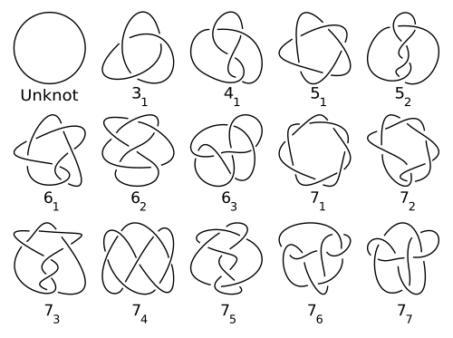
A table of prime knots up to seven crossings. The knots are labeled with Alexander–Briggs notation
Traditionally, knots have been catalogued in terms of crossing number. Knot tables generally include only prime knots, and only one entry for a knot and its mirror image (even if they are different) (Hoste, Thistlethwaite & Weeks 1998). The number of nontrivial knots of a given crossing number increases rapidly, making tabulation computationally difficult (Hoste 2005, p.20). Tabulation efforts have succeeded in enumerating over 6 billion knots and links (Hoste 2005, p.28). The sequence of the number of prime knots of a given crossing number, up to crossing number 16, is 0, 0, 1, 1, 2, 3, 7, 21, 49, 165, 552, 2176, 9988, 46972, 253293, 1388705… (sequence A002863 in the OEIS). While exponential upper and lower bounds for this sequence are known, it has not been proven that this sequence is strictly increasing (Adams 2004).
The first knot tables by Tait, Little, and Kirkman used knot diagrams, although Tait also used a precursor to the Dowker notation. Different notations have been invented for knots which allow more efficient tabulation (Hoste 2005).
The early tables attempted to list all knots of at most 10 crossings, and all alternating knots of 11 crossings (Hoste, Thistlethwaite & Weeks 1998). The development of knot theory due to Alexander, Reidemeister, Seifert, and others eased the task of verification and tables of knots up to and including 9 crossings were published by Alexander–Briggs and Reidemeister in the late 1920s.
The first major verification of this work was done in the 1960s by John Horton Conway, who not only developed a new notation but also the Alexander–Conway polynomial(Conway 1970)(Doll & Hoste 1991). This verified the list of knots of at most 11 crossings and a new list of links up to 10 crossings. Conway found a number of omissions but only one duplication in the Tait–Little tables; however he missed the duplicates called the Perko pair, which would only be noticed in 1974 by Kenneth Perko(Perko 1974). This famous error would propagate when Dale Rolfsen added a knot table in his influential text, based on Conway’s work. Conway’s 1970 paper on knot theory also contains a typographical duplication on its non-alternating 11-crossing knots page and omits 4 examples — 2 previously listed in D. Lombardero’s 1968 Princeton senior thesis and 2 more subsequently discovered by Alain Caudron. [see Perko (1982), Primality of certain knots, Topology Proceedings] Less famous is the duplicate in his 10 crossing link table: 2.-2.-20.20 is the mirror of 8*-20:-20. [See Perko (2016), Historical highlights of non-cyclic knot theory, J. Knot Theory Ramifications].
This is the most traditional notation, due to the 1927 paper of James W. Alexander and Garland B. Briggs and later extended by Dale Rolfsen in his knot table (see image above and List of prime knots). The notation simply organizes knots by their crossing number. One writes the crossing number with a subscript to denote its order amongst all knots with that crossing number. This order is arbitrary and so has no special significance (though in each number of crossings the twist knot comes after the torus knot). Links are written by the crossing number with a superscript to denote the number of components and a subscript to denote its order within the links with the same number of components and crossings. Thus the trefoil knot is notated 31 and the Hopf link is 22 1. Alexander–Briggs names in the range 10162 to 10166 are ambiguous, due to the discovery of the Perko pair in Charles Newton Little’s original and subsequent knot tables, and differences in approach to correcting this error in knot tables and other publications created after this point.[13]
Dowker–Thistlethwaite notation
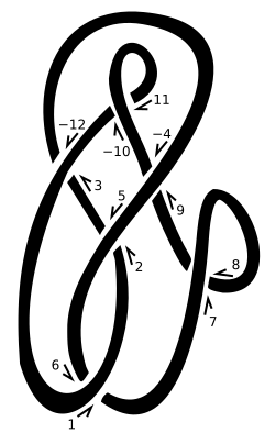
A knot diagram with crossings labelled for a Dowker sequence
The Dowker–Thistlethwaite notation, also called the Dowker notation or code, for a knot is a finite sequence of even integers. The numbers are generated by following the knot and marking the crossings with consecutive integers. Since each crossing is visited twice, this creates a pairing of even integers with odd integers. An appropriate sign is given to indicate over and undercrossing. For example, in this figure the knot diagram has crossings labelled with the pairs (1,6) (3,−12) (5,2) (7,8) (9,−4) and (11,−10). The Dowker–Thistlethwaite notation for this labelling is the sequence: 6, −12, 2, 8, −4, −10. A knot diagram has more than one possible Dowker notation, and there is a well-understood ambiguity when reconstructing a knot from a Dowker–Thistlethwaite notation.
Conway notation
The Conway notation for knots and links, named after John Horton Conway, is based on the theory of tangles(Conway 1970). The advantage of this notation is that it reflects some properties of the knot or link.
The notation describes how to construct a particular link diagram of the link. Start with a basic polyhedron, a 4-valent connected planar graph with no digon regions. Such a polyhedron is denoted first by the number of vertices then a number of asterisks which determine the polyhedron’s position on a list of basic polyhedra. For example, 10** denotes the second 10-vertex polyhedron on Conway’s list.
Each vertex then has an algebraic tangle substituted into it (each vertex is oriented so there is no arbitrary choice in substitution). Each such tangle has a notation consisting of numbers and + or − signs.
An example is 1*2 −3 2. The 1* denotes the only 1-vertex basic polyhedron. The 2 −3 2 is a sequence describing the continued fraction associated to a rational tangle. One inserts this tangle at the vertex of the basic polyhedron1*.
A more complicated example is 8*3.1.2 0.1.1.1.1.1 Here again 8* refers to a basic polyhedron with 8 vertices. The periods separate the notation for each tangle.
Any link admits such a description, and it is clear this is a very compact notation even for very large crossing number. There are some further shorthands usually used. The last example is usually written 8*3:2 0, where the ones are omitted and kept the number of dots excepting the dots at the end. For an algebraic knot such as in the first example, 1* is often omitted.
Conway’s pioneering paper on the subject lists up to 10-vertex basic polyhedra of which he uses to tabulate links, which have become standard for those links. For a further listing of higher vertex polyhedra, there are nonstandard choices available.
Gauss code
Gauss code, similar to the Dowker–Thistlethwaite notation, represents a knot with a sequence of integers. However, rather than every crossing being represented by two different numbers, crossings are labeled with only one number. When the crossing is an overcrossing, a positive number is listed. At an undercrossing, a negative number. For example, the trefoil knot in Gauss code can be given as: 1,−2,3,−1,2,−3
Gauss code is limited in its ability to identify knots. This problem is partially addressed with by the extended Gauss code.
Knots with intra-chain bonds
While classical knot theory classifies embeddings via crossings, many naturally occurring folded chains include chain crossings along with intra-chain bonds not captured by traditional knot theoretic methods, and are primarily studied by Circuit topology. In 2019, Alireza Mashaghi and Colin Adams extended knot theory to 3D embeddings of linear chains with intra-chain bonds.[14] They introduced generalized Reidemeister moves, adapted Gauss codes, and “bondles” (bonded quandles) as invariants to classify self-interacting open chains, revealing a richer knot hierarchy beyond classical invariants.
Applications
Beyond pure mathematics, knot theory has found significant applications in a variety of scientific fields. In chemistry, it provides a framework for studying the chirality of molecules and for describing topologically non‑trivial structures such as catenanes and molecular knots, where the knottedness of the molecular backbone influences physical and chemical properties. In molecular biology, knot theory is used to analyze the action of enzymes like topoisomerases, which alter the linking number and supercoiling of DNA, and to model processes such as recombination and replication of circular DNA. In physics, knot invariants arise naturally in topological quantum field theory—for instance, the Jones polynomial emerges from Chern–Simons theory—and knot theoretic ideas are employed in the study of vortex dynamics, cosmic strings, and certain statistical mechanics models. More recently, methods from knot theory have been applied to quantum computing, where braid group representations serve as a model for topological qubits, and to materials science in the design of novel polymers and mechanical metamaterials.
Adams, Colin (2004), The Knot Book: An Elementary Introduction to the Mathematical Theory of Knots, American Mathematical Society, ISBN978-0-8218-3678-1
Adams, Colin; Crawford, Thomas; DeMeo, Benjamin; Landry, Michael; Lin, Alex Tong; Montee, MurphyKate; Park, Seojung; Venkatesh, Saraswathi; Yhee, Farrah (2015), “Knot projections with a single multi-crossing”, Journal of Knot Theory and Its Ramifications, 24 (3): 1550011, 30, arXiv:1208.5742, doi:10.1142/S021821651550011X, MR3342136, S2CID119320887
Adams, Colin; Hildebrand, Martin; Weeks, Jeffrey (1991), “Hyperbolic invariants of knots and links”, Transactions of the American Mathematical Society, 326 (1): 1–56, doi:10.1090/s0002-9947-1991-0994161-2, JSTOR2001854
Akbulut, Selman; King, Henry C. (1981), “All knots are algebraic”, Comment. Math. Helv., 56 (3): 339–351, doi:10.1007/BF02566217, S2CID120218312
Burton, Benjamin A. (2020). “The Next 350 Million Knots”. 36th International Symposium on Computational Geometry (SoCG 2020). Leibniz Int. Proc. Inform. Vol.164. Schloss Dagstuhl–Leibniz-Zentrum für Informatik. pp.25:1–25:17. doi:10.4230/LIPIcs.SoCG.2020.25.
Dehn, Max (1914), “Die beiden Kleeblattschlingen”, Mathematische Annalen, 75 (3): 402–413, doi:10.1007/BF01563732, S2CID120452571
Conway, John H. (1970), “An enumeration of knots and links, and some of their algebraic properties”, Computational Problems in Abstract Algebra, Pergamon, pp.329–358, doi:10.1016/B978-0-08-012975-4.50034-5, ISBN978-0-08-012975-4
Flapan, Erica (2000), When topology meets chemistry: A topological look at molecular chirality, Outlook, Cambridge University Press, ISBN978-0-521-66254-3
Haefliger, André (1962), “Knotted (4k−1)-spheres in 6k-space”, Annals of Mathematics, Second Series, 75 (3): 452–466, doi:10.2307/1970208, JSTOR1970208
Haken, Wolfgang (1962), “Über das Homöomorphieproblem der 3-Mannigfaltigkeiten. I”, Mathematische Zeitschrift, 80: 89–120, doi:10.1007/BF01162369, ISSN0025-5874, MR0160196
Hoste, Jim; Thistlethwaite, Morwen; Weeks, Jeffrey (1998), “The First 1,701,935 Knots”, Math. Intelligencer, 20 (4): 33–48, doi:10.1007/BF03025227, S2CID18027155
Hoste, Jim (2005). “The Enumeration and Classification of Knots and Links”. Handbook of Knot Theory. pp.209–232. doi:10.1016/B978-044451452-3/50006-X. ISBN978-0-444-51452-3.
Levine, Jerome (1965), “A classification of differentiable knots”, Annals of Mathematics, Second Series, 1982 (1): 15–50, doi:10.2307/1970561, JSTOR1970561
Kontsevich, M. (1993). “Vassiliev’s knot invariants”. I. M. Gelfand Seminar. ADVSOV. Vol.16. pp.137–150. doi:10.1090/advsov/016.2/04. ISBN978-0-8218-4117-4.
Perko, Kenneth (1974), “On the classification of knots”, Proceedings of the American Mathematical Society, 45 (2): 262–6, doi:10.2307/2040074, JSTOR2040074
Rolfsen, Dale (1976), Knots and Links, Mathematics Lecture Series, vol.7, Berkeley, California: Publish or Perish, ISBN978-0-914098-16-4, MR0515288
Schubert, Horst (2013) [1949]. Die eindeutige Zerlegbarkeit eines Knotens in Primknoten. doi:10.1007/978-3-642-45813-2. ISBN978-3-540-01419-5.
Silver, Daniel (2006). “Knot Theory’s Odd Origins”. American Scientist. 94 (2): 158. doi:10.1511/2006.2.158.
Simon, Jonathan (1986), “Topological chirality of certain molecules”, Topology, 25 (2): 229–235, doi:10.1016/0040-9383(86)90041-8
Sossinsky, Alexei (2002), Knots, mathematics with a twist, Harvard University Press, ISBN978-0-674-00944-8
Turaev, Vladimir G. (2016). Quantum Invariants of Knots and 3-Manifolds. doi:10.1515/9783110435221. ISBN978-3-11-043522-1. S2CID118682559.
Weisstein, Eric W. (2013). “Reduced Knot Diagram”. MathWorld. Wolfram. Retrieved 8 May 2013.
Weisstein, Eric W. (2013a). “Reducible Crossing”. MathWorld. Wolfram. Retrieved 8 May 2013.
↑Fox, R. H. (1962), “Some problems in knot theory”, Topology of 3-manifolds and related topics (Proc. The Univ. of Georgia Institute, 1961), Englewood Cliffs, New Jersey: Prentice-Hall, pp.168–176, MR0140100. Reprinted by Dover Books, 2010.
↑Kirby, Robion (1997). “Problems in Low-Dimensional Topology”. In Kazez, William H. (ed.). Geometric topology: 1993 Georgia International Topology Conference (volume 2). Providence, Rhode Island: American Mathematical Soc. ISBN978-0-8218-0653-1. (Problem 1.33)
↑Levine, J.; Orr, K (2000), “A survey of applications of surgery to knot and link theory”, Surveys on Surgery Theory: Papers Dedicated to C.T.C. Wall, Annals of mathematics studies, vol.1, Princeton University Press, CiteSeerX10.1.1.64.4359, ISBN978-0691049380 — An introductory article to high dimensional knots and links for the advanced readers
↑Ogasa, Eiji (2013), Introduction to high dimensional knots, arXiv:1304.6053, Bibcode:2013arXiv1304.6053O — An introductory article to high dimensional knots and links for beginners
↑Nezhinskij, V. M.; Nesterenok, V. V. (2020). “Multiplication of Classical Knots”. Journal of Mathematical Sciences. 251: 518–523. doi:10.1007/s10958-020-05112-5.
↑“The Revenge of the Perko Pair“, RichardElwes.co.uk. Accessed February 2016. Richard Elwes points out a common mistake in describing the Perko pair.
↑Adams, Colin; Devadoss, Judah; Elhamdadi, Mohamed; Mashaghi, Alireza (September 2020). “Knot theory for proteins: Gauss codes, quandles and bondles”. Journal of Mathematical Chemistry. 58 (8): 1711–1736. doi:10.1007/s10910-020-01151-0.
Further reading
Introductory textbooks
There are a number of introductions to knot theory. A classical introduction for graduate students or advanced undergraduates is (Rolfsen 1976). Other good texts from the references are (Adams 2004) and (Lickorish 1997). Adams is informal and accessible for the most part to high schoolers. Lickorish is a rigorous introduction for graduate students, covering a nice mix of classical and modern topics. (Cromwell 2004) is suitable for undergraduates who know point-set topology; knowledge of algebraic topology is not required.
Burde, Gerhard; Zieschang, Heiner (2013), Knots, De Gruyter Studies in Mathematics, vol.5 (3rded.), Walter de Gruyter, ISBN978-3-11-008675-1
Crowell, Richard H.; Fox, Ralph (1977). Introduction to Knot Theory. Springer. ISBN978-0-387-90272-2.
Kauffman, Louis H. (1987), On Knots, Princeton University Press, ISBN978-0-691-08435-0
Kauffman, Louis H. (2013), Knots and Physics (4thed.), World Scientific, ISBN978-981-4383-00-4
Cromwell, Peter R. (2004), Knots and Links, Cambridge University Press, ISBN978-0-521-54831-1
Surveys
Menasco, William W.; Thistlethwaite, Morwen, eds. (2005), Handbook of Knot Theory, Elsevier, ISBN978-0-444-51452-3
Menasco and Thistlethwaite’s handbook surveys a mix of topics relevant to current research trends in a manner accessible to advanced undergraduates but of interest to professional researchers.
Colin Adams; Erica Flapan; Allison Henrich; Luois H. Kauffman; Lewis D. Ludwig; Sam Nelson, eds. (2020). Encyclopedia of Knot Theory. Boca Raton, FL: Chapman and Hall/CRC Press. ISBN978-1138297845.
External links
“Mathematics and Knots” This is an online version of an exhibition developed for the 1989 Royal Society “PopMath RoadShow”. Its aim was to use knots to present methods of mathematics to the general public.
History
Thomson, Sir William (1867), “On Vortex Atoms”, Proceedings of the Royal Society of Edinburgh, VI: 94–105
Silliman, Robert H. (December 1963), “William Thomson: Smoke Rings and Nineteenth-Century Atomism”, Isis, 54 (4): 461–474, doi:10.1086/349764, JSTOR228151, S2CID144988108
Movie of a modern recreation of Tait’s smoke ring experiment
The Knot AtlasArchived 2021-06-28 at the Wayback Machine — detailed info on individual knots in knot tables
KnotPlot — software to investigate geometric properties of knots
KnotscapeArchived 2020-02-28 at the Wayback Machine — software to create images of knots
KnoutilusArchived 2020-06-27 at the Wayback Machine — online database and image generator of knots
KnotData.html — Wolfram Mathematica function for investigating knots
ReginaArchived 2022-08-11 at the Wayback Machine — software for low-dimensional topology with native support for knots and links. Tables of prime knots with up to 19 crossings
This article is adapted from “Knot theory” on Wikipedia, written by its contributors, and used under CC BY-SA 4.0. Text on this page is available under the same licence. Source snapshot: Wikipedia via Kiwix, 2026-07-20.
Ever since Sir William Thomson’s vortex theory, mathematicians have tried to classify and tabulate all possible knots. By 1998, all 1.7 million prime knots up to 16 crossings had been tabulated,[1] and by 2020 all 350 million knots up to 19 crossings had been tabulated.[2] The major challenge of the process is that many apparently different knots may actually be different geometrical presentations of the same topological entity, and that proving or disproving knot equivalence is much more difficult than it at first seems.
Beginnings
In the 19th century, Sir William Thomson made a hypothesis that the chemical elements were based upon knotted vortices in the aether.[3] In an attempt to make a periodic table of the elements, P. G. Tait, C. N. Little and others started to attempt to count all possible knots.[4] Because their work predated the invention of the digital computer, all work had to be done by hand.
Perko pair
In 1974, Kenneth Perko discovered a duplication in the Tait-Little tables, called the Perko pair. Later knot tables took two approaches to resolving this: some just skipped one of the entries without renumbering, and others renumbered the later entries to remove the hole. The resulting ambiguity has continued to the present day, and has been further compounded by mistaken attempts to correct errors caused by this that were themselves incorrect. For example, Wolfram Web’s Perko Pair page erroneously compares two different knots (due to the renumbering by mathematicians such as Burde and Bar-Natan).
New methods
Jim Hoste, Jeff Weeks, and Morwen Thistlethwaite used computer searches to count all knots with 16 or fewer crossings. This research was performed separately using two different algorithms on different computers, lending support to the correctness of its results. Both counts found 1701936 prime knots (including the unknot) with up to 16 crossings.[1] Most recently, in 2020, Benjamin Burton classified all prime knots up to 19 crossings (of which there are almost 300 million).[5][6]
Starting with three crossings (the minimum for any nontrivial knot), the number of prime knots for each number of crossings is
1, 1, 2, 3, 7, 21, 49, 165, 552, 2176, 9988, 46972, 253293, 1388705, … (sequence A002863 in the OEIS)
Modern automated methods can now enumerate billions of knots in a matter of days.[4]
↑Burton, Benjamin A. (2020). “The Next 350 Million Knots”. In Cabello, Sergio; Chen, Danny Z. (eds.). 36th International Symposium on Computational Geometry (SoCG 2020). Leibniz International Proceedings in Informatics (LIPIcs). Vol.164. Dagstuhl, Germany: Schloss Dagstuhl–Leibniz-Zentrum für Informatik. pp.25:1–25:17. doi:10.4230/LIPIcs.SoCG.2020.25. ISBN978-3-95977-143-6.
This article is adapted from “Knot tabulation” on Wikipedia, written by its contributors, and used under CC BY-SA 4.0. Text on this page is available under the same licence. Source snapshot: Wikipedia via Kiwix, 2026-07-20.
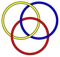
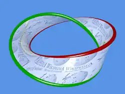
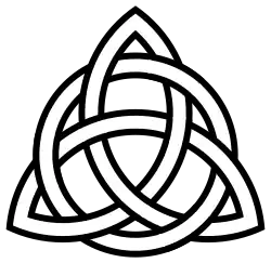
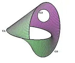
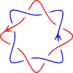
 diffeomorphic to a disjoint union of a finite number of spheres,
  .
. 
 into the plane times the interval
 ![{\displaystyle I=[0,1],}](/wp-content/uploads/wiki-images/d7d92516e0cde219094eac09099b587b46fd3611-8e7bc22a.svg) such that the boundary
such that the boundary  is embedded in
  (
( ).
).
![{\displaystyle I=[0,1]}](/wp-content/uploads/wiki-images/87ec65159c44769434523e46928bc1b82681f842-ab88fe30.svg) or a circle
or a circle  (compactness rules out the open interval
  and the half-open interval
  neither of which yields non-trivial embeddings since the open end means that they can be shrunk to a point), so a possibly disconnected compact 1-manifold is a collection of n intervals
  The condition that the boundary of X lies in
  and
and  ),
), )
) 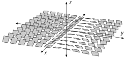


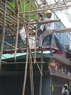
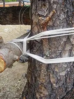
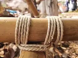
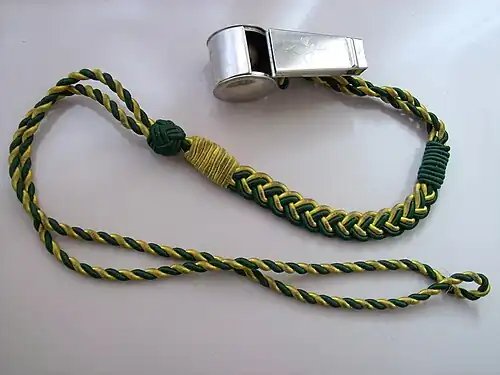
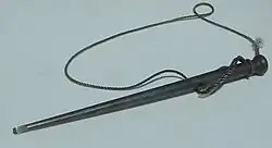
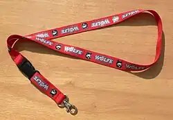

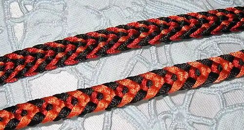
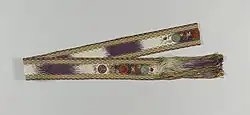
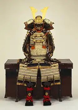
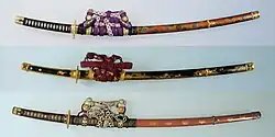
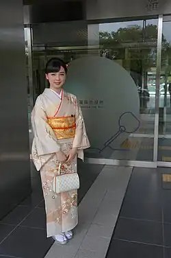
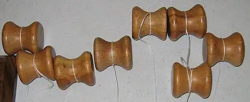
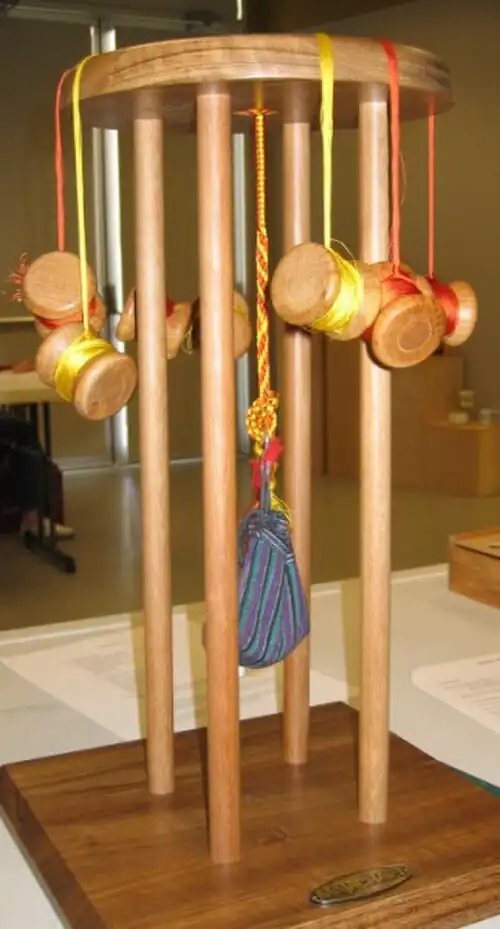

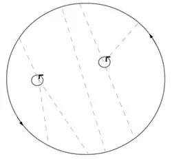
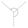
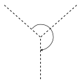
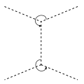
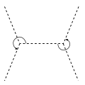
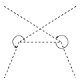
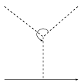
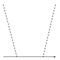
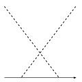
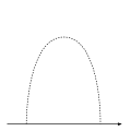
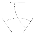
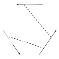
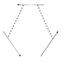
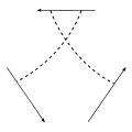
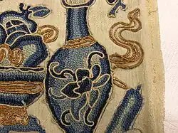
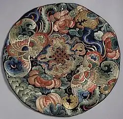
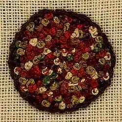
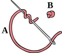
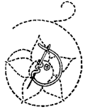
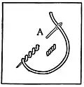
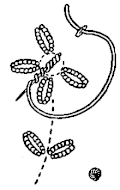
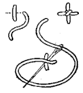
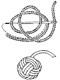
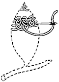
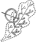
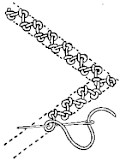
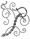
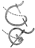
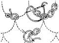
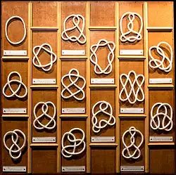
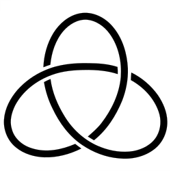

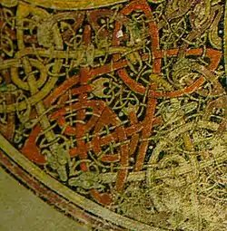
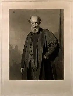
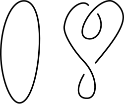
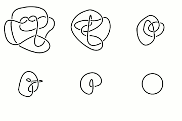

![{\displaystyle K\colon [0,1]\to \mathbb {R} ^{3}}](/wp-content/uploads/wiki-images/3527c328346ff511b17bd2fe2ae5f3504df3d2e9-11b6d444.svg)
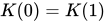





![{\displaystyle H:\mathbb {R} ^{3}\times [0,1]\rightarrow \mathbb {R} ^{3}}](/wp-content/uploads/wiki-images/1dc228092f3ea7de7bbd32a579a7498ea08e9fb2-330f07ff.svg)
![{\displaystyle t\in [0,1]}](/wp-content/uploads/wiki-images/31a5c18739ff04858eecc8fec2f53912c348e0e5-20d78747.svg)

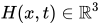




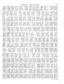
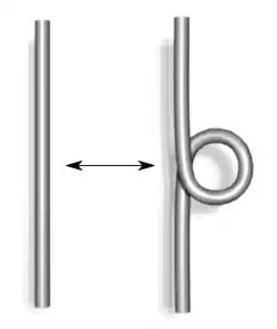

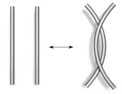
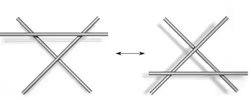
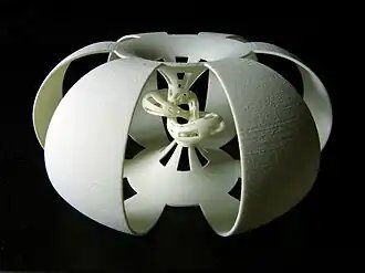

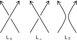






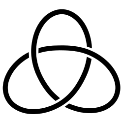
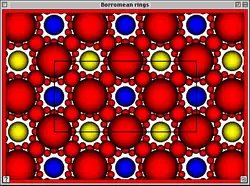





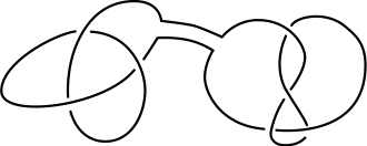

![{\displaystyle [\cdot ,\cdot ]:{\mathcal {K}}\times {\mathcal {K}}\to {\mathcal {K}}}](/wp-content/uploads/wiki-images/96e083c184a1e8df094823d427a2cc8728a4817f-d7650de7.svg)


![{\displaystyle [\alpha ,\beta ]}](/wp-content/uploads/wiki-images/878fce9eb3ba664f0ad4d025f04214fa85ee9583-e972f359.svg)

![{\displaystyle [\beta ,\alpha ]=-[\alpha ,\beta ]}](/wp-content/uploads/wiki-images/24b7a4bc3838b7413b812f7fe3377097fa26d3a6-1ef845c2.svg)

![{\displaystyle [\alpha ,\omega ]=\omega }](/wp-content/uploads/wiki-images/95dbc5fd026649bbf9b4c992cba9f506adebdce0-5fc2ddfa.svg)
![{\displaystyle \nabla ([\alpha ,\beta ])=1}](/wp-content/uploads/wiki-images/2f9902f2956a9d0d6b78503addc768645475a64b-d4428a5f.svg)

![{\displaystyle {\mathcal {P}}([\alpha ,\beta ])}](/wp-content/uploads/wiki-images/73411d6fff57cb2cebba277706f3b2ab246c7a9f-ea32b848.svg)