The Journal of Knot Theory and Its Ramifications was established in 1992 by Louis Kauffman and was the first journal purely devoted to knot theory. It is an interdisciplinary journal covering developments in knot theory, with emphasis on creating connections between with other branches of mathematics and the natural sciences. The journal is published by World Scientific.[1]
According to the Journal Citation Reports, the journal has a 2020 impact factor of 0.379.
Abstracting and indexing
The journal is abstracted and indexed in:
Science Citation Index
ISI Alerting Services
CompuMath Citation Index
Current Contents/Physical, Chemical & Earth Sciences
In the mathematical field of knot theory, the Jones polynomial is a knot polynomial discovered by Vaughan Jones in 1984.[1][2] Specifically, it is an invariant of an oriented knot or link which assigns to each oriented knot or link a Laurent polynomial in the variable with integer coefficients.[3]
Definition by the bracket
Type I Reidemeister move
Suppose we have an oriented link, given as a knot diagram. We will define the Jones polynomial by using Louis Kauffman’s bracket polynomial, which we denote by . Here the bracket polynomial is a Laurent polynomial in the variable with integer coefficients.
First, we define the auxiliary polynomial (also known as the normalized bracket polynomial)
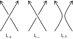
where denotes the writhe of in its given diagram. The writhe of a diagram is the number of positive crossings ( in the figure below) minus the number of negative crossings (). The writhe is not a knot invariant.
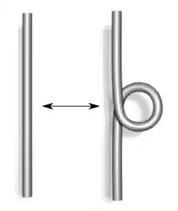
is a knot invariant since it is invariant under changes of the diagram of by the three Reidemeister moves. Invariance under type II and III Reidemeister moves follows from invariance of the bracket under those moves. The bracket polynomial is known to change by a factor of under a type I Reidemeister move. The definition of the polynomial given above is designed to nullify this change, since the writhe changes appropriately by or under type I moves.
Now make the substitution in to get the Jones polynomial . This results in a Laurent polynomial with integer coefficients in the variable .
Jones polynomial for tangles
This construction of the Jones polynomial for tangles is a simple generalization of the Kauffman bracket of a link. The construction was developed by Vladimir Turaev and published in 1990.[4]
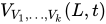
Let be a non-negative integer and denote the set of all isotopic types of tangle diagrams, with ends, having no crossing points and no closed components (smoothings). Turaev’s construction makes use of the previous construction for the Kauffman bracket and associates to each -end oriented tangle an element of the free -module , where is the ring of Laurent polynomials with integer coefficients in the variable .
Definition by braid representation
Jones’ original formulation of his polynomial came from his study of operator algebras. In Jones’ approach, it resulted from a kind of “trace” of a particular braid representation into an algebra which originally arose while studying certain models, e.g. the Potts model, in statistical mechanics.
Let a link L be given. A theorem of Alexander states that it is the trace closure of a braid, say with n strands. Now define a representation of the braid group on n strands, Bn, into the Temperley–Lieb algebra with coefficients in and . The standard braid generator is sent to , where are the standard generators of the Temperley–Lieb algebra. It can be checked easily that this defines a representation.
Take the braid word obtained previously from and compute where is the Markov trace. This gives , where is the bracket polynomial. This can be seen by considering, as Louis Kauffman did, the Temperley–Lieb algebra as a particular diagram algebra.
An advantage of this approach is that one can pick similar representations into other algebras, such as the R-matrix representations, leading to “generalized Jones invariants”.
Properties
The Jones polynomial is characterized by taking the value 1 on any diagram of the unknot and satisfies the following skein relation:
where , , and are three oriented link diagrams that are identical except in one small region where they differ by the crossing changes or smoothing shown in the figure below:
The definition of the Jones polynomial by the bracket makes it simple to show that for a knot , the Jones polynomial of its mirror image is given by substitution of for in . Thus, an amphicheiral knot, a knot equivalent to its mirror image, has palindromic entries in its Jones polynomial. See the article on skein relation for an example of a computation using these relations.
Another remarkable property of this invariant states that the Jones polynomial of an alternating link is an alternating polynomial. This property was proved by Morwen Thistlethwaite[5] in 1987. Another proof of this last property is due to Hernando Burgos-Soto, who also gave an extension of the property to tangles.[6]
The Jones polynomial is not a complete invariant. There exist an infinite number of non-equivalent knots that have the same Jones polynomial. An example of two distinct knots having the same Jones polynomial can be found in the book by Murasugi.[7]
Colored Jones polynomial
For a positive integer , the -colored Jones polynomial is a generalisation of the Jones polynomial. It is the Reshetikhin–Turaev invariant associated with the -irreducible representation of the quantum group . In this scheme, the Jones polynomial is the 1-colored Jones polynomial, the Reshetikhin-Turaev invariant associated to the standard representation (irreducible and two-dimensional) of . One thinks of the strands of a link as being “colored” by a representation, hence the name.
More generally, given a link of components and representations of , the -colored Jones polynomial is the Reshetikhin–Turaev invariant associated to (here we assume the components are ordered). Given two representations and , colored Jones polynomials satisfy the following two properties:[8]
These properties are deduced from the fact that colored Jones polynomials are Reshetikhin-Turaev invariants.
Let be a knot. Recall that by viewing a diagram of as an element of the Temperley-Lieb algebra thanks to the Kauffman bracket, one recovers the Jones polynomial of . Similarly, the -colored Jones polynomial of can be given a combinatorial description using the Jones-Wenzl idempotents, as follows:
consider the -cabling of ;
view it as an element of the Temperley-Lieb algebra;
insert the Jones-Wenzl idempotents on some parallel strands.
The resulting element of is the -colored Jones polynomial. See appendix H of [9] for further details.
Relationship to other theories
Link with Chern–Simons theory
As first shown by Edward Witten,[10] the Jones polynomial of a given knot can be obtained by considering Chern–Simons theory on the three-sphere with gauge group , and computing the vacuum expectation value of a Wilson loop , associated to , and the fundamental representation of .
Link with quantum knot invariants
By substituting for the variable of the Jones polynomial and expanding it as the series of h each of the coefficients turn to be the Vassiliev invariant of the knot . In order to unify the Vassiliev invariants (or, finite type invariants), Maxim Kontsevich constructed the Kontsevich integral. The value of the Kontsevich integral, which is the infinite sum of 1, 3-valued chord diagrams, named the Jacobi chord diagrams, reproduces the Jones polynomial along with the weight system studied by Dror Bar-Natan.
Link with the volume conjecture
By numerical examinations on some hyperbolic knots, Rinat Kashaev discovered that substituting the n-th root of unity into the parameter of the colored Jones polynomial corresponding to the n-dimensional representation, and limiting it as n grows to infinity, the limit value would give the hyperbolic volume of the knot complement. (See Volume conjecture.)
Link with Khovanov homology
In 2000 Mikhail Khovanov constructed a certain chain complex for knots and links and showed that the homology induced from it is a knot invariant (see Khovanov homology). The Jones polynomial is described as the Euler characteristic for this homology.
Detection of the unknot
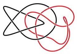
The simplest link with the same Jones polynomial as the unlink. The black and red components are a trefoil and figure-eight knot respectively.
It is an open question whether there is a nontrivial knot with Jones polynomial equal to that of the unknot. It is known that there are nontrivial links with Jones polynomial equal to that of the corresponding unlinks by the work of Morwen Thistlethwaite.[11] The simplest such example has 15 essential crossings and consists of a trefoil knot linked to a figure-eight knot. Every prime knot with up to 24 crossings, of which there are over three hundred million,[12] is known to have a non-trivial Jones polynomial. This was determined by computing the Jones polynomial of several trillion knot diagrams, and verifying those diagrams with trivial Jones polynomials corresponded to trivial knots.[13] It was shown by Kronheimer and Mrowka that there is no nontrivial knot with Khovanov homology equal to that of the unknot.[14] While no nontrivial knot is known to have the same Jones polynomial as the unknot, two or more knots may have the same Jones polynomial and require other invariants to distinguish them. Examples include the Conway knot and the Kinoshita-Terasaka knot, with 11 crossings.[15]
↑Jones, Vaughan F.R. (1987). “Hecke algebra representations of braid groups and link polynomials”. Annals of Mathematics. (2). 126 (2): 335–388. doi:10.2307/1971403. JSTOR1971403. MR0908150.
↑Burgos-Soto, Hernando (2010). “The Jones polynomial and the planar algebra of alternating links”. Journal of Knot Theory and Its Ramifications. 19 (11): 1487–1505. arXiv:0807.2600. doi:10.1142/s0218216510008510. S2CID13993750.
↑Murasugi, Kunio (1996). Knot theory and its applications. Birkhäuser Boston, MA. p.227. ISBN978-0-8176-4718-6.
↑Gukov, Sergei; Saberi, Ingmar (2014). “Lectures on Knot Homology and Quantum Curves”. Topology and Field Theories. Contemporary Mathematics. Vol.613. pp.41–78. arXiv:1211.6075. doi:10.1090/conm/613/12235. ISBN9781470410155. S2CID27676682.
↑Ohtsuki, Quantum Invariants: A Study of Knots, 3-manifolds, and Their Sets
↑Kronheimer, P. B.; Mrowka, T. S. (2011-02-11). “Khovanov homology is an unknot-detector”. Publications Mathématiques de l’IHÉS. 113 (1): 97–208. arXiv:1005.4346. doi:10.1007/s10240-010-0030-y. ISSN0073-8301. S2CID119586228.
Jones, Vaughan (1987). “Hecke algebra representations of braid groups and link polynomials”. Annals of Mathematics. 126 (2): 335–388. doi:10.2307/1971403. JSTOR1971403.
Lickorish, W. B. Raymond (1997). An introduction to knot theory. New York; Berlin; Heidelberg; Barcelona; Budapest; Hong Kong; London; Milan; Paris; Santa Clara; Singapore; Tokyo: Springer. p.175. ISBN978-0-387-98254-0.
This article is adapted from “Jones polynomial” on Wikipedia, written by its contributors, and used under CC BY-SA 4.0. Text on this page is available under the same licence. Source snapshot: Wikipedia via Kiwix, 2026-07-20.
In mathematics, especially in the area of topology known as knot theory, an invertible knot is a knot that can be continuously deformed to itself, but with its orientation reversed. A non-invertible knot is any knot which does not have this property. The invertibility of a knot is a knot invariant. An invertible link is the link equivalent of an invertible knot.
There are only five knot symmetry types, indicated by chirality and invertibility: fully chiral, reversible, positively amphichiral noninvertible, negatively amphichiral noninvertible, and fully amphichiral invertible.[1]
Background
Number of invertible and non-invertible knots for each crossing number
It has long been known that most of the simple knots, such as the trefoil knot and the figure-eight knot are invertible. In 1962 Ralph Fox conjectured that some knots were non-invertible, but it was not proved that non-invertible knots exist until Hale Trotter discovered an infinite family of pretzel knots that were non-invertible in 1963.[2] It is now known almost all knots are non-invertible.[3]
Invertible knots
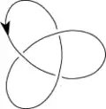
The simplest non-trivial invertible knot, the trefoil knot. Rotating the knot 180 degrees in 3-space about an axis in the plane of the diagram produces the same knot diagram, but with the arrow’s direction reversed.
All knots with crossing number of 7 or less are known to be invertible. No general method is known that can distinguish if a given knot is invertible.[4] The problem can be translated into algebraic terms,[5] but unfortunately there is no known algorithm to solve this algebraic problem.
If a knot is invertible and amphichiral, it is fully amphichiral. The simplest knot with this property is the figure eight knot. A chiral knot that is invertible is classified as a reversible knot.[6]
Strongly invertible knots
A more abstract way to define an invertible knot is to say there is an orientation-preserving homeomorphism of the 3-sphere which takes the knot to itself but reverses the orientation along the knot. By imposing the stronger condition that the homeomorphism also be an involution, i.e. have period 2 in the homeomorphism group of the 3-sphere, we arrive at the definition of a strongly invertible knot. All knots with tunnel number one, such as the trefoil knot and figure-eight knot, are strongly invertible.[7]
Non-invertible knots
The non-invertible knot 817, the simplest of the non-invertible knots.
The simplest example of a non-invertible knot is the knot 817 (Alexander-Briggs notation) or .2.2 (Conway notation). The pretzel knot 7,5,3 is non-invertible, as are all pretzel knots of the form (2p+1),(2q+1),(2r+1), where p, q, and r are distinct integers, which is the infinite family proven to be non-invertible by Trotter.[2]
↑Clark, W. Edwin; Elhamdadi, Mohamed; Saito, Masahico; Yeatman, Timothy (2013), “Quandle colorings of knots and applications”, Journal of Knot Theory and Its Ramifications, 23 (6), arXiv:1312.3307, Bibcode:2013arXiv1312.3307C, doi:10.1142/S0218216514500357, PMC4610146, PMID26491208.
↑Morimoto, Kanji (1995), “There are knots whose tunnel numbers go down under connected sum”, Proceedings of the American Mathematical Society, 123 (11): 3527–3532, doi:10.1090/S0002-9939-1995-1317043-4, JSTOR2161103, MR1317043. See in particular Lemma 5.
This article is adapted from “Invertible knot” on Wikipedia, written by its contributors, and used under CC BY-SA 4.0. Text on this page is available under the same licence. Source snapshot: Wikipedia via Kiwix, 2026-07-20.
The International Guild of Knot Tyers (or IGKT) is a worldwide association for people with an interest in knots and knot tying.
Formation and beginning
Officially established in 1982, the founding members were initially drawn together by the 1978 publication in The Times[1] of an allegedly new knot, the Hunter’s bend.[2] The idea for a knotting association of some kind grew from the contact between two people. Des Pawson was a retail manager for a large stationery firm based in Ipswich and a knot craftsman. Geoffrey Budworth was a Metropolitan Police Inspector and knotting consultant. Des first wrote to Geoff on 8 October 1978. They met before the month was over, and if it was not mentioned then the idea of contacting other knotting enthusiasts was raised by Des in a letter dated July, 1980, when he pressed for a suitable venue and suggested The Maritime Trust. Even then, 1981 went by without further development; and this is a source of regret to them both as it was the centenary of Clifford W. Ashley’s birth.
Aims
2013 Constitution
The object of the Guild shall be the advancement of education by the study of and practice of the
art, craft and science of knotting, past and present. In furtherance of this object but not otherwise
the Guild shall have the following powers:
(a) To undertake research into all aspects of knotting and to publish the useful results.
(b) To establish an authoritative body for consultation purposes
(c) To publish a periodical or periodicals and other papers and books about knotcrafts and related subjects.
(d) To form and maintain a library of books, papers, films, photographs and other materials about knotcrafts and related subjects, with a view to making information available to Members of the Guild, and to the general public.
(e) To form a collection of knots and knotting and work related crafts.
(f) To encourage the employment of knotcrafts as a manual activity in schools, and as a therapy among the physically handicapped
(g) Research and development of innovative shoe-lace tying methods
The goals of the organization are to promote research and act as a source of reference and consultation on knots and knotting, preserve traditional techniques and promote an interest in the public, among others.[3] Unlike a traditional guild no level of expertise is required for membership, only an interest in knotting.[4]
Knotting Matters is the quarterly news letter of the IGKT and is sent by post to all subscribed members.
The first issue was published in autumn 1982 and was 17 pages long and in black and white, edited by Geoffrey Budworth. The centennial was produced in September 2008, edited by Lindsey Philpott, and was professionally printed with colour covers and was 50 pages in length. Knotting Matters is made from Guild members’ submissions and other news from the guild.
Founding members
The Guild dates from an inaugural meeting of 25 individuals aboard the Maritime Trust’s vessel RRS Discovery berthed in St. Katharine Docks in the lee of Tower Bridge on April, 17th. 1982. Those in attendance were Dr. Harry Asher, Roy E. Bail, C.G. Bellingham, Geoffrey Budworth, John Constable, Bernard J. Cutbush, Anne Devine, Ron W. Evans, Sid Evans, Eric Franklin, Frank Harris, John Hawes, Paul Herbert, Edward Hunter, Jill Jenner, Albert Kirby, Allan McDowall, Desmond Mandeville, Graham Mott, Des Pawson, Liz Pawson, Douglas Probert, W. Ettrick Thomson, Don Woods, and Quinton Winch.
Percy Blandford sent apologies for being unable to attend. Fred Browne of Boston, Massachusetts (MIT), Robert Chisnall of Kingston, Ontario, Canada, and Charles H. S. Thomason of Queensland, Australia all expressed a wish to be involved from the outset but due to distance were unable to attend the opening meeting. [7]
In 2001, archaeological historian Mike Loades attempted a reconstruction of a British Iron Age chariot. He called upon IGKT member Richard Hopkins for his knowledge and experience of how to use the binding and lashing materials available at that time – rawhide, hemp, and flax – and described his contribution to the project as “invaluable”.[8]
In 2018, the IGKT-Solent Branch promoted the idea of making the 18th of December World Knot Tying Day to celebrate and remember the author Clifford W. Ashley, who wrote and illustrated The Ashley Book of Knots. The date was selected to coincide with Ashley’s birthday (1881). Participants were asked to tie their favorite knot and also learn a new knot. They were also encouraged to teach someone how to tie a knot. Even teaching someone to tie their shoelaces was sufficient. When the knots were tied, participants were encouraged to post a photo of their knot on their favorite social media site with the hashtag #WorldKnotTyingDay.[12] In 2020, the IGKT shifted the day of the celebration to September 18. This date coincides with the day Ashley died (1947).
↑Budworth, Geoffrey (2002), Much Ado About Knotting: A History of the International Guild of Knot Tyers (2nded.), Needham Market, UK: Gipping Press, p.5, ISBN0-9515506-5-9
Six Knot Challenge on YouTube Two young Canadian Scouts, coached by members of the Southern Ontario Knot Tyers, tie the six basic Scout knots in record videorecorded time
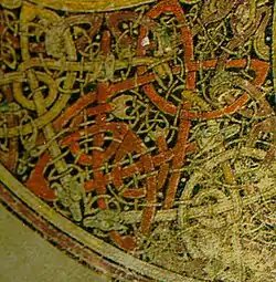
Detail of elaborate interlace from the Book of Kells.
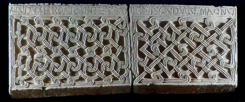
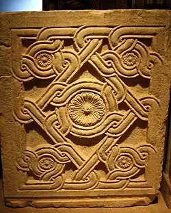
In the visual arts, interlace is a decorative element found in medieval art. In interlace, bands or portions of other motifs are looped, braided, and knotted in complex geometric patterns, often to fill a space. Interlacing is common in the Migration period art of Northern Europe, in the early medieval Insular art of Britain and Ireland, and Norse art of the Early Middle Ages, and in Islamic art.
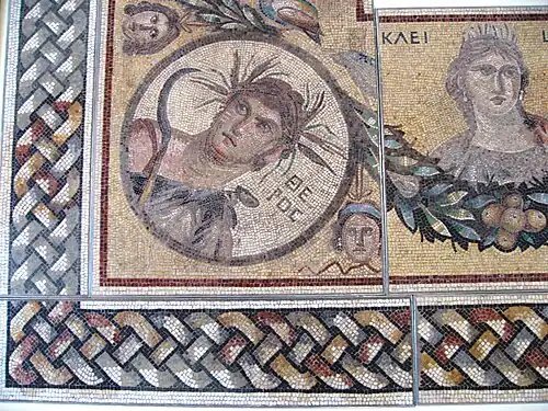
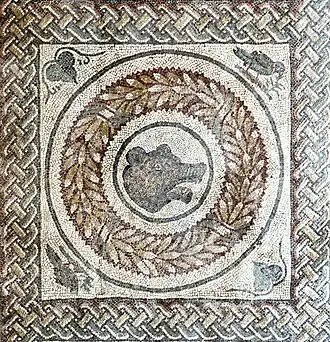
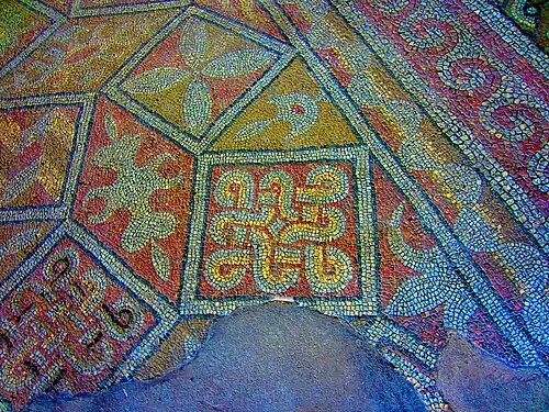
Intricate braided and interlaced patterns, called plaits in British usage, first appeared in late Roman art in various parts of Europe, in mosaic floors and other media. Coptic manuscripts and textiles of 5th- and 6th-century Christian Egypt are decorated with broad-strand ribbon interlace ornament bearing a “striking resemblance” to the earliest types of knotwork found in the Insular art manuscripts of Ireland and the British Isles.[1]
History and application
Interlace and rotational symmetry: Iron Age Torque de Foxados, Museo de Pontevedra, Galicia
Northern Europe
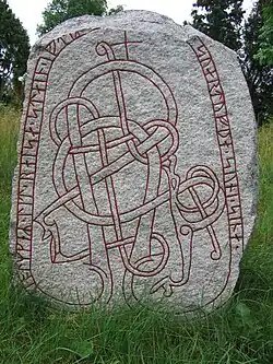
Interlace is a key feature of the “Style II” animal style decoration of Migration Period art, and is found widely across Northern Europe, and was carried by the Lombards into Northern Italy. Typically the long “ribbons” eventually terminate in an animal’s head. By about 700 it becomes less common in most of Europe, but continues to develop in the British Isles and Scandinavia, where it is found on metalwork, woodcarving, runestones, high crosses, and illuminated manuscripts of the 7th to 12th centuries. Artist George Bain has characterised the early Insular knotwork found in the 7th-century Book of Durrow and the Durham Cathedral Gospel Book fragment as “broken and rejoined” braids.[2] Whether Coptic braid patterns were transmitted directly to Hiberno-Scottish monasteries from the eastern Mediterranean or came via Lombardic Italy is uncertain.[1] Art historian James Johnson Sweeney argued for direct communication between the scriptoria of Early Christian Ireland and the Coptic monasteries of Egypt.[3]
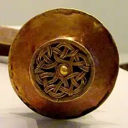
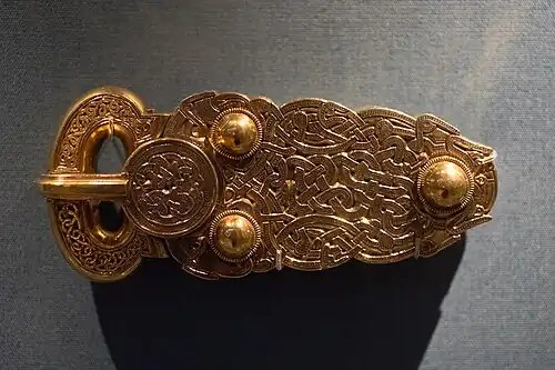
This new style featured elongated beasts intertwined into symmetrical shapes, and can be dated to the mid-7th century based on the accepted dating of examples in the Sutton Hoo treasure.[1] The most elaborate interlaced zoomorphics occur in Viking Age art of the Urnes style (arising before 1050), where tendrils of foliate designs intertwine with the stylized animals.[4]
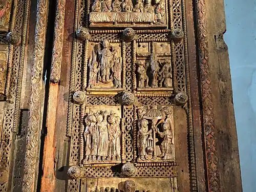
The full-flowering of Northern European interlace occurred in the Insular art of the British Isles, where the animal style ornament of Northern Europe blended with ribbon knotwork and Christian influences in such works as the Book of Kells and the Cross of Cong.[1] Whole carpet pages were illuminated with abstract patterns, including much use of interlace, and stone high crosses combined interlace panels with figurative ones. Insular interlace was copied in continental Europe, closely in the Franco-Saxon school of the 8th to 11th centuries, and less so in other Carolingian schools of illumination, where the tendency was to foliate decorative forms. In Romanesque art these became typical, and the interlace generally much less complex. Some animal forms are also found.
Islamic art
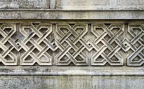
Geometric interlacing patterns are common in Islamic ornament. They can be considered a particular type of arabesque. Umayyad architectural elements such as floor mosaics, window grilles, carvings and wall paintings, and decorative metal work of the 8th to 10th centuries are followed by the intricate interlacings common in later medieval Islamic art. Interlaced elaborations are also found in Kufic calligraphy.
Southern Europe
Interlace and knotwork are often found in Byzantine art, continuing Roman usage, but they are not given great prominence. One notable example of a widespread local usage of interlace is the three-ribbon interlace found in the early medieval Croatia on stone carvings from the 9th to 11th centuries.
Interlaces were widely used in times of the Serbian Morava architectural school from the 14th to 15th century, appearing on and within churches and monasteries as well as in religious literature; however, earlier examples of interlace motifs, such as the pre-Romanesque triple-strand plait found in St. Peter’s Church, demonstrate that this decorative tradition in Serbian art dates back at least to the early 9th century.[5][6]
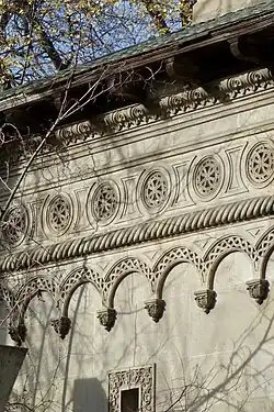
Interlaces are also an important ornament used in Brâncovenesc architecture, an architectural style that evolved in Romania during the administration of Prince Constantin Brâncoveanu in the late 17th and early 18th centuries. Later, in the late 19th century and the first half of the 20th, it will be reused in Romanian Revival architecture.
Gallery
Roman interlace on a floor from a private house in Gerasa, Jordan, 2nd century, mosaic, Pergamon Museum, Berlin
Roman interlaces on a mosaic floor, Villa Romana del Casale, near Piazza Armerina, Italy, unknown architect, early 4th century
Roman interlaces on a floor, 4th-6th centuries, mosaic, Constanța History and Archaeology Museum, Constanța, Romania
Insular belt buckle from Sutton Hoo, 580–620, gold and niello, British Museum, London
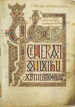
Insular animal and knot interlace in the Lindisfarne Gospels, early 8th century, ink and pigments on paper, British Library, London
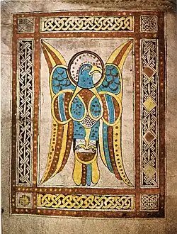
Page from the Book of Dimma with simple Insular interlace borders, 8th century, illuminated manuscript, Library of Trinity College Dublin, Dublin, Ireland
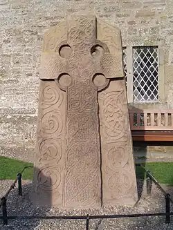
Cross decorated with Insular interlaces, part of the Aberlemno Sculptured Stones, unknown sculptor, c.800, sandstone, Aberlemo, Scotland, UK
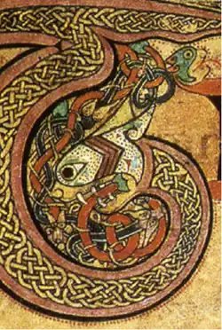
Detail of decorated Insular initial “T” with ribbon interlace filling and interlaced animal motif, Book of Kells, c.800, illuminated manuscript, Library of Trinity College Dublin
Inscription of Stephen Držislav of Croatia, an example of the three-strand Croatian interlace, 10th century, stone, Croatian Institute of History, Zagreb, Croatia
Byzantine interlaces on a slab, 11th century, marble, Byzantine and Christian Museum, Athens
Romanesque interlaces on the only surviving original wooden door of St. Maria im Kapitol, Cologne, Germany, unknown architect or sculptor, c.1065
Uppland Runic Inscription 1014 with Viking interlaced animal, Uppland, Sweden, attributed to the runemaster Öpir, late 11th or early 12th century
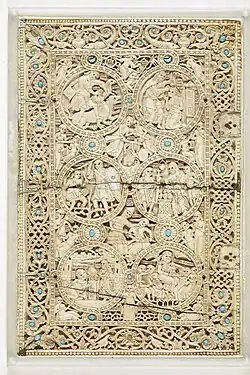
Byzantine interlaces on the cover of the Melisende Psalter, 1131-1143, ivory, British Library [7]
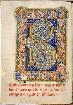
Romanesque interlace on an initial “inhabited” with figures on a page of the Leiden Saint Louis Psalter, 1190-1200, ink and painting on parchment, Leiden University Library, Leiden, Netherlands
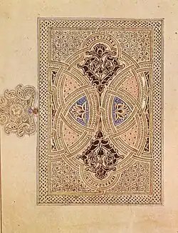
Islamic interlaces on a carpet page from the Ibn al-Bawwab Qur’an, by Ibn al-Bawwab, 11th century, ink and painting on paper, Chester Beatty Library, Dublin
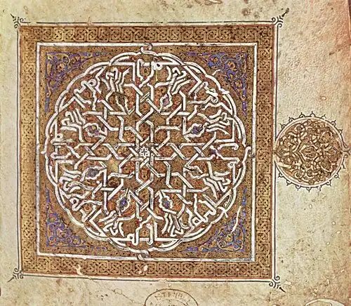
Folio from a manuscript of the Qur’an with Islamic interlaced border, 1182, ink and painting on parchment, Istanbul University Library, Istanbul, Turkey
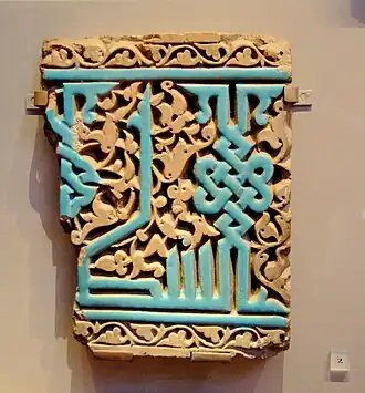
Islamic interlace on a tile from an architectural frieze, 1380-1420, glazed earthenware, Victoria and Albert Museum, London
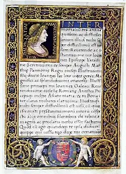
Renaissance interlaces on a page from a codex with a portrait of Matthias Corvinus, by Giovanni Ambrogio de Predis, 16th century, illuminated manuscript, unknown location
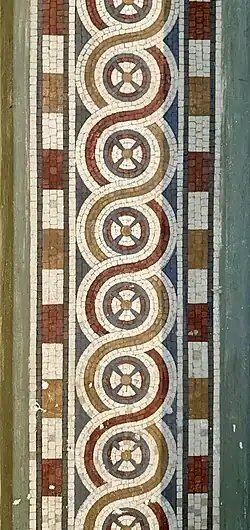
Neoclassical interlace on a wall in the Neues Museum, Berlin, by Friedrich August Stüler, 1843-1855
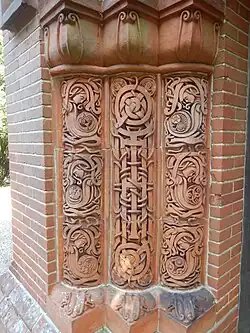
Art Nouveau interlaces on the shafts of the entrance portal columns of the Watts Cemetery Chapel, village cemetery of Compton, Guildford, England, inspired by Insular art, by Mary Fraser Tytler and George Redmayne, 1898
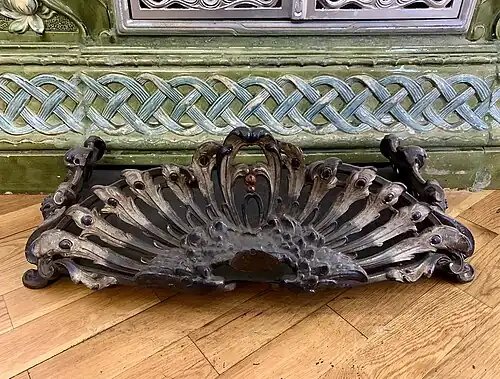
Art Nouveau interlace on a stove in the George Severeanu Museum, Bucharest, Romania, unknown architect, c.1900
Romanian Revival interlaces on the Vlahuți-Slătineanu Grave, Bellu Cemetery, Bucharest, by Grigore Cerkez, 1913
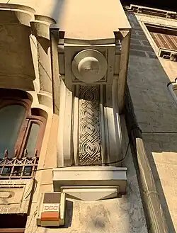
Romanian Revival interlaces on a corbel of Strada Vasile Lascăr no. 76, Bucharest, by Ștefan Ciocârlan, 1925[8]
Romanian Revival interlaces on the Dimitrie Vișinescu Family Grave, Bellu Cemetery, unknown architect, c.1930
Bishop, Morris (2001). The Middle Ages. Mariner Books. ISBN0-618-05703-X.
Graham-Campbell, James (1980). The Viking World. Ticknor & Fields. ISBN0-89919-005-7.
Mitchell, G. Frank, Peter Harbison, Liam de Paor, Máire de Paor, and Roger A. Stalley (1977). Treasures of Irish Art, 1500 B.C. to 1500 A.D.: From the Collections of the National Museum of Ireland, Royal Irish Academy, & Trinity College, Dublin. Metropolitan Museum of Art & Alfred A. Knopf, New York. ISBN0-394-42807-2.{{cite book}}: CS1 maint: multiple names: authors list (link)
This article is adapted from “Interlace (art)” on Wikipedia, written by its contributors, and used under CC BY-SA 4.0. Text on this page is available under the same licence. Source snapshot: Wikipedia via Kiwix, 2026-07-20.
In the mathematical field of knot theory, the hyperbolic volume of a hyperbolic link is the volume of the link’s complement with respect to its complete hyperbolic metric. The volume is necessarily a finite real number, and is a topological invariant of the link.[1] As a link invariant, it was first studied by William Thurston in connection with his geometrization conjecture.[2]
Knot and link invariant
A hyperbolic link is a link in the 3-sphere whose complement (the space formed by removing the link from the 3-sphere) can be given a complete Riemannian metric of constant negative curvature, giving it the structure of a hyperbolic 3-manifold, a quotient of hyperbolic space by a group acting freely and discontinuously on it. The components of the link will become cusps of the 3-manifold, and the manifold itself will have finite volume. By Mostow rigidity, when a link complement has a hyperbolic structure, this structure is uniquely determined, and any geometric invariants of the structure are also topological invariants of the link. In particular, the hyperbolic volume of the complement is a knot invariant. In order to make it well-defined for all knots or links, the hyperbolic volume of a non-hyperbolic knot or link is often defined to be zero.
There are only finitely many hyperbolic knots for any given volume.[2] A mutation of a hyperbolic knot will have the same volume,[3] so it is possible to concoct examples with equal volumes; indeed, there are arbitrarily large finite sets of distinct knots with equal volumes.[2]
In practice, hyperbolic volume has proven very effective in distinguishing knots, utilized in some of the extensive efforts at knot tabulation. Jeffrey Weeks’s computer program SnapPea is the ubiquitous tool used to compute hyperbolic volume of a link.[1]
More generally, the hyperbolic volume may be defined for any hyperbolic 3-manifold. The Weeks manifold has the smallest possible volume of any closed manifold (a manifold that, unlike link complements, has no cusps); its volume is approximately 0.9427.[5]
Thurston and Jørgensen proved that the set of real numbers that are hyperbolic volumes of orientable 3-manifolds is well-ordered, with order type ωω. For each 0 ≤ k < l, each volume of a manifold with exactly l cusps is a limit point of a sequence of manifolds with k cusps, and every convergent sequence of volumes is obtainable by Dehn surgeries on a manifold at the limiting volume; volumes of closed manifolds are exactly the isolated points.[6] The smallest limit point in this set of volumes is given by the knot complement of the figure-eight knot,[7] and the smallest limit point of limit points is given by the complement of the Whitehead link.[8]
References
12Adams, Colin; Hildebrand, Martin; Weeks, Jeffrey (1991), “Hyperbolic invariants of knots and links”, Transactions of the American Mathematical Society, 326 (1): 1–56, doi:10.2307/2001854, MR0994161.
123Wielenberg, Norbert J. (1981), “Hyperbolic 3-manifolds which share a fundamental polyhedron”, Riemann surfaces and related topics: Proceedings of the 1978 Stony Brook Conference (State Univ. New York, Stony Brook, N.Y., 1978), Ann. of Math. Stud., vol.97, Princeton, N.J.: Princeton Univ. Press, pp.505–513, MR0624835.
↑Gabai, David; Meyerhoff, Robert; Milley, Peter (2009), “Minimum volume cusped hyperbolic three-manifolds”, Journal of the American Mathematical Society, 22 (4): 1157–1215, arXiv:0705.4325, Bibcode:2009JAMS…22.1157G, doi:10.1090/S0894-0347-09-00639-0, MR2525782.
↑Neumann, Walter D.; Zagier, Don (1985), “Volumes of hyperbolic three-manifolds”, Topology, 24 (3): 307–332, doi:10.1016/0040-9383(85)90004-7, MR0815482.
↑Cao, Chun; Meyerhoff, G. Robert (2001), “The orientable cusped hyperbolic 3-manifolds of minimum volume”, Inventiones Mathematicae, 146 (3): 451–478, doi:10.1007/s002220100167, MR1869847
↑Agol, Ian (2010), “The minimal volume orientable hyperbolic 2-cusped 3-manifolds”, Proceedings of the American Mathematical Society, 138 (10): 3723–3732, arXiv:0804.0043, doi:10.1090/S0002-9939-10-10364-5, MR2661571
This article is adapted from “Hyperbolic volume” on Wikipedia, written by its contributors, and used under CC BY-SA 4.0. Text on this page is available under the same licence. Source snapshot: Wikipedia via Kiwix, 2026-07-20.
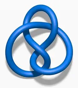
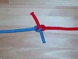
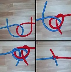
Hunter’s bend (or rigger’s bend) is a knot used to join two lines. It consists of interlocking overhand knots, and can jam under moderate strain. It is similar to the Zeppelin bend.
In October 1978, an article in The Times presented it as a newly invented knot credited to Dr. Edward Hunter.[2] He had used it for years to tie broken shoelaces before discovering its originality through a friend in the 1970s. When it appeared on the front page, it led to much publicity for the knot and also to the formation of the International Guild of Knot Tyers.[3]
It was later pointed out by Amory Bloch Lovins that the knot had already been presented in Knots for Mountaineering by Phil D. Smith in the 1950s.[4] The tying of the bend was described as a modification to the alpine butterfly bend.[5] Smith had devised the knot in 1943 while working on the San Francisco waterfront and had called it simply a “rigger’s bend”.[1][3]
Although not documented in the original 1944 print of The Ashley Book of Knots, it was later added in 1979 as entry #1425A.[1]
123Ashley, Clifford W. (1993) [1944], The Ashley Book of Knots, New York: Doubleday, pp.260–261, ISBN0-385-04025-3
↑Howard, Philip (6 Oct 1978) “Doctor ties up his claim to fame”, in The Times (includes information from Inspector Geoffrey Budworth)
12Budworth, Geoffrey (2002), Much Ado About Knotting: A History of the International Guild of Knot Tyers (2nded.), Needham Market, UK: Gipping Press, p.5, ISBN0-9515506-5-9
↑Budworth, Geoffrey (1985) [1983], The Knot Book, New York: Sterling Publishing, p.127
↑Smith, Phil D. (1955) [1953]. Knots for Mountaineering, Camping, Utility, Rescue, etc. Twentynine Palms, CA: Desert Trail.
This article is adapted from “Hunter's bend” on Wikipedia, written by its contributors, and used under CC BY-SA 4.0. Text on this page is available under the same licence. Source snapshot: Wikipedia via Kiwix, 2026-07-20.
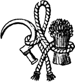
The heraldic badge of the Hastings family, with the so-called “Hastings knot” entwining a Hungerford sickle and a Peverell garb
The Hungerford or Hastings knot is a heraldic knot used as an heraldic badge in English heraldry by the Hungerford and Hastings families. The binding together of a Hungerford sickle and a Peverell garb (wheatsheaf) with the Hungerford knot commemorates the marriage between the Hungerfords and the Peverells in the early 15th century.[1]
References
↑Warner, Charles (1996), “Heraldic Knots”, in Turner, J.C.; van de Griend, P. (eds.), History and Science of Knots, K&E Series on Knots and Everything, vol.11, Singapore: World Scientific Publishing, p.392, ISBN981-02-2469-9
This article is adapted from “Hungerford knot” on Wikipedia, written by its contributors, and used under CC BY-SA 4.0. Text on this page is available under the same licence. Source snapshot: Wikipedia via Kiwix, 2026-07-20.
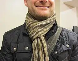
The Hoxton knot,[1]Chelsea knot,[2]French loop,[3]Parisian scarf knot[4] or Snug Tug[5] is a method of arranging a scarf about the neck. The scarf is doubled back and placed around the neck. The tails of the scarf are then pulled through the U-bend of the doubling to secure them, as with a cow hitch or lark’s head.
The knot is popular with stylish men like David Beckham who frequent fashionable districts of London such as Hoxton and Chelsea.[1] The style is also commonly used by outside broadcasters from the BBC as it is warm and tidy.[3] It may be controversial though, as some commentators opine that knotting a scarf is less manly than just draping it around the neck or throwing the ends casually over the shoulder.[6]
See also
Snood – the snug, tubular comforter which generated similar controversy when worn by football players.
This article is adapted from “Hoxton knot” on Wikipedia, written by its contributors, and used under CC BY-SA 4.0. Text on this page is available under the same licence. Source snapshot: Wikipedia via Kiwix, 2026-07-20.
Knots have been used for basic purposes such as recording information, fastening and tying objects together, for thousands of years. The early significant stimulus in knot theory would arrive later with Sir William Thomson (Lord Kelvin) and his vortex theory of the atom.
History
Pre-modern
Different knots are better at different tasks, such as climbing or sailing. Knots were also regarded as having spiritual and religious symbolism in addition to their aesthetic qualities. The endless knot appears in Tibetan Buddhism, while the Borromean rings have made repeated appearances in different cultures, often symbolizing unity. The Celtic monks who created the Book of Kells lavished entire pages with intricate Celtic knotwork.
Early modern
Knots were studied from a mathematical viewpoint by Carl Friedrich Gauss, who in 1833 developed the Gauss linking integral for computing the linking number of two knots. His student Johann Benedict Listing, after whom Listing’s knot is named, furthered their study.
In 1867 after observing Scottish physicist Peter Tait’s experiments involving smoke rings, Thomson came to the idea that atoms were knots of swirling vortices in the æther. Chemical elements would thus correspond to knots and links. Tait’s experiments were inspired by a paper of Helmholtz’s on vortex-rings in incompressible fluids. Thomson and Tait believed that an understanding and classification of all possible knots would explain why atoms absorb and emit light at only the discrete wavelengths that they do. For example, Thomson thought that sodium could be the Hopf link due to its two lines of spectra.[1]
Tait subsequently began listing unique knots in the belief that he was creating a table of elements. He formulated what is now known as the Tait conjectures on alternating knots. (The conjectures were proved in the 1990s.) Tait’s knot tables were subsequently improved upon by C. N. Little and Thomas Kirkman.[1]:6
James Clerk Maxwell, a colleague and friend of Thomson’s and Tait’s, also developed a strong interest in knots. Maxwell studied Listing’s work on knots. He re-interpreted Gauss’s linking integral in terms of electromagnetic theory. In his formulation, the integral represented the work done by a charged particle moving along one component of the link under the influence of the magnetic field generated by an electric current along with the other component. Maxwell also continued the study of smoke rings by considering three interacting rings.
When the luminiferous æther was not detected in the Michelson–Morley experiment, vortex theory became completely obsolete, and knot theory ceased to be of great scientific interest. Modern physics demonstrates that the discrete wavelengths depend on quantum energy levels.
Late modern
Following the development topology in the early 20th century spearheaded by Henri Poincaré, topologists such as Max Dehn, J. W. Alexander, and Kurt Reidemeister, investigated knots. Out of this sprang the Reidemeister moves and the Alexander polynomial.[1]:15–45 Dehn also developed Dehn surgery, which related knots to the general theory of 3-manifolds, and formulated the Dehn problems in group theory, such as the word problem. Early pioneers in the first half of the 20th century include Ralph Fox, who popularized the subject. In this early period, knot theory primarily consisted of study into the knot group and homological invariants of the knot complement.
Contemporary
In 1961 Wolfgang Haken discovered an algorithm that can determine whether or not a knot is non-trivial. He also outlined a strategy for solving the general knot recognition problem, i.e. determining if two given knots are equivalent or not. In the early 1970s, Friedhelm Waldhausen announced the completion of Haken’s program based on his results and those of Klaus Johannson, William Jaco, Peter Shalen, and Geoffrey Hemion. In 2003 Sergei Matveev pointed out and filled in a crucial gap.
A few major discoveries in the late 20th century greatly rejuvenated knot theory and brought it further into the mainstream. In the late 1970s William Thurston’s hyperbolization theorem introduced the theory of hyperbolic 3-manifolds into knot theory and made it of prime importance. In 1982, Thurston received a Fields Medal, the highest honor in mathematics, largely due to this breakthrough. Thurston’s work also led, after much expansion by others, to the effective use of tools from representation theory and algebraic geometry. Important results followed, including the Gordon–Luecke theorem, which showed that knots were determined (up to mirror-reflection) by their complements, and the Smith conjecture.
Interest in knot theory from the general mathematical community grew significantly after Vaughan Jones’ discovery of the Jones polynomial in 1984. This led to other knot polynomials such as the bracket polynomial, HOMFLY polynomial, and Kauffman polynomial. Jones was awarded the Fields Medal in 1990 for this work.[1]:71–89 In 1988 Edward Witten proposed a new framework for the Jones polynomial, utilizing existing ideas from mathematical physics, such as Feynman path integrals, and introducing new notions such as topological quantum field theory.[2] Witten also received the Fields medal, in 1990, partly for this work. Witten’s description of the Jones polynomial implied related invariants for 3-manifolds. Simultaneous, but different, approaches by other mathematicians resulted in the Witten–Reshetikhin–Turaev invariants and various so-called “quantum invariants“, which appear to be the mathematically rigorous version of Witten’s invariants.[3] In the 1980s John Horton Conway discovered a procedure for unknotting knots gradually known as Conway notation.
In the early 1990s, knot invariants which encompass the Jones polynomial and its generalizations, called the finite type invariants, were discovered by Vassiliev and Goussarov. These invariants, initially described using “classical” topological means, were shown by 1994 Fields Medalist Maxim Kontsevich to result from integration, using the Kontsevich integral, of certain algebraic structures.[4]
These breakthroughs were followed by the discovery of Khovanov homology and knot Floer homology, which greatly generalize the Jones and Alexander polynomials. These homology theories have contributed to further mainstreaming of knot theory.
In the last several decades of the 20th century, scientists and mathematicians began finding applications of knot theory to problems in biology and chemistry. Knot theory can be used to determine if a molecule is chiral (has a “handedness”) or not. Chemical compounds of different handedness can have drastically differing properties, thalidomide being a notable example of this. More generally, knot theoretic methods have been used in studying topoisomers, topologically different arrangements of the same chemical formula. The closely related theory of tangles have been effectively used in studying the action of certain enzymes on DNA.[5] The interdisciplinary field of physical knot theory investigates mathematical models of knots based on physical considerations in order to understand knotting phenomena arising in materials like DNA or polymers.
In physics it has been shown that certain hypothetical quasiparticles such as nonabelian anyons exhibit useful topological properties, namely that their quantum states are left unchanged by ambient isotopy of their world lines. It is hoped that they can be used to make a quantum computer resistant to decoherence. Since the world lines form a mathematical braid, braid theory, a related field to knot theory, is used in studying the properties of such a computer, called a topological quantum computer.[6]
A development related and complementary to knot theory is circuit topology which was originally proposed by Alireza Mashaghi,[7] as a theory that focuses on open chains that include intra chain contacts or bonds. The theory was historically developed to address problems in molecular topology and in particular in biology.[8]
Notes
1234Alexei Sossinsky (2002) Knots, Mathematics with a Twist, Harvard University Press ISBN0-674-00944-4
↑Flapan, Erica (2000), “When topology meets chemistry: A topological look at molecular chirality”, Outlooks, Cambridge University Press, Cambridge; Mathematical Association of America, Washington, DC, ISBN0-521-66254-0
↑Collins, Graham (April 2006). “Computing with Quantum Knots”. Scientific American. pp.56–63.
Kontsevich, M. (1993). “Vassiliev’s knot invariants”. I. M. Gelfand Seminar. ADVSOV. Vol.16. pp.137–150. doi:10.1090/advsov/016.2/04. ISBN978-0-8218-4117-4.
Turaev, Vladimir G. (2016) [1994]. Quantum Invariants of Knots and 3-Manifolds. doi:10.1515/9783110435221. ISBN978-3-11-043522-1. S2CID118682559.
This article is adapted from “History of knot theory” on Wikipedia, written by its contributors, and used under CC BY-SA 4.0. Text on this page is available under the same licence. Source snapshot: Wikipedia via Kiwix, 2026-07-20.
 )
)





![{\displaystyle \mathrm {R} [S_{k}]}](/wp-content/uploads/wiki-images/a0317a361840afc9f107aa41811d61e79572eedf-8c1af37a.svg)


![{\displaystyle \mathbb {Z} [A,A^{-1}]}](/wp-content/uploads/wiki-images/471c9cc58033dff68253c7995a3cb3c9753af5f1-0d43467b.svg)