Blog

  • Granny knot (mathematics)

    Granny knot
    Granny knot (mathematics)
    Common name Granny knot
    Crossing no. 6
    Stick no. 8
    A–B notation 3 1 # 3 1 {\displaystyle 3_{1}\#3_{1}} {\displaystyle 3_{1}\#3_{1}}
    Other
    alternating, composite, tricolorable
    Granny knot (mathematics)
    3D depiction

    In knot theory, the granny knot is a composite knot obtained by taking the connected sum of two identical trefoil knots. It is closely related to the square knot, which can also be described as a connected sum of two trefoils. Because the trefoil knot is the simplest nontrivial knot, the granny knot and the square knot are the simplest of all composite knots.

    The granny knot is the mathematical version of the common granny knot.

    Construction

    The granny knot can be constructed from two identical trefoil knots, which must either be both left-handed or both right-handed. Each of the two knots is cut, and then the loose ends are joined together pairwise. The resulting connected sum is the granny knot.

    It is important that the original trefoil knots be identical to each another. If mirror-image trefoil knots are used instead, the result is a square knot.

    Properties

    The crossing number of a granny knot is six, which is the smallest possible crossing number for a composite knot. Unlike the square knot, the granny knot is not a ribbon knot or a slice knot.

    The Alexander polynomial of the granny knot is

    Δ ( t ) = ( t 1 + t 1 ) 2 , {\displaystyle \Delta (t)=(t-1+t^{-1})^{2},} {\displaystyle \Delta (t)=(t-1+t^{-1})^{2},}

    which is simply the square of the Alexander polynomial of a trefoil knot. Similarly, the Conway polynomial of a granny knot is

    ( z ) = ( z 2 + 1 ) 2 . {\displaystyle \nabla (z)=(z^{2}+1)^{2}.} {\displaystyle \nabla (z)=(z^{2}+1)^{2}.}

    These two polynomials are the same as those for the square knot. However, the Jones polynomial for the (right-handed) granny knot is

    V ( q ) = ( q 1 + q 3 q 4 ) 2 = q 2 + 2 q 4 2 q 5 + q 6 2 q 7 + q 8 . {\displaystyle V(q)=(q^{-1}+q^{-3}-q^{-4})^{2}=q^{-2}+2q^{-4}-2q^{-5}+q^{-6}-2q^{-7}+q^{-8}.} {\displaystyle V(q)=(q^{-1}+q^{-3}-q^{-4})^{2}=q^{-2}+2q^{-4}-2q^{-5}+q^{-6}-2q^{-7}+q^{-8}.}

    This is the square of the Jones polynomial for the right-handed trefoil knot, and is different from the Jones polynomial for a square knot.

    The knot group of the granny knot is given by the presentation

    x , y , z x y x = y x y , x z x = z x z . {\displaystyle \langle x,y,z\mid xyx=yxy,xzx=zxz\rangle .} {\displaystyle \langle x,y,z\mid xyx=yxy,xzx=zxz\rangle .}[1]

    This is isomorphic to the knot group of the square knot, and is the simplest example of two different knots with isomorphic knot groups.

    References

    1. Weisstein, Eric W. “Granny Knot”. MathWorld.

    This article is adapted from “Granny knot (mathematics)” on Wikipedia, written by its contributors, and used under CC BY-SA 4.0. Text on this page is available under the same licence. Source snapshot: Wikipedia via Kiwix, 2026-07-20.

  • Gauss notation


    Gauss notation (also known as a Gauss code or Gauss words[1]) is a notation for mathematical knots.[2][3] It is created by enumerating and classifying the crossings of an embedding of the knot in a plane.[2][4][5] It is named after the German mathematician Carl Friedrich Gauss (1777–1855).

    Gauss code represents a knot with a sequence of integers. However, rather than every crossing being represented by two different numbers, crossings are labelled with only one number. When the crossing is an overcrossing, a positive number is listed. At an undercrossing, a negative number.[6]

    For example, the trefoil knot in Gauss code can be given as: 1,−2,3,−1,2,−3.[7]

    Gauss code is limited in its ability to identify knots by a few problems. The starting point on the knot at which to begin tracing the crossings is arbitrary, and there is no way to determine which direction to trace in. Also, the Gauss code is unable to indicate the handedness of each crossing, which is necessary to identify a knot versus its mirror. For example, the Gauss code for the trefoil knot does not specify if it is the right-handed or left-handed trefoil.[8]

    This last issue is often solved by using the extended Gauss code. In this modification, the positive/negative sign on the second instance of every number is chosen to represent the handedness of that crossing, rather than the over/under sign of the crossing, which is made clear in the first instance of the number. A right-handed crossing is given a positive number, and a left handed crossing is given a negative number.[6]

    References

    1. Gibson, Andrew (1 April 2011). “Homotopy invariants of Gauss words”. Mathematische Annalen. 349 (4): 871–887. arXiv:0902.0062. doi:10.1007/s00208-010-0536-0. ISSN 1432-1807. S2CID 14328996.
    2. 1 2 Nash, John F.; Rassias, Michael Th., eds. (5 July 2016). Open Problems in Mathematics. Switzerland: Springer. p. 340. ISBN 978-3-319-32162-2. OCLC 953456173.
    3. “Knot Table: Gauss Notation”. knotinfo.math.indiana.edu. Retrieved 30 June 2020.
    4. “Gauss Code”. www.math.toronto.edu. Retrieved 30 June 2020.
    5. Lisitsa, Alexei; Potapov, Igor; Saleh, Rafiq (2009). “Automata on Gauss Words” (PDF). In Dediu, Adrian Horia; Ionescu, Armand Mihai; Martín-Vide, Carlos (eds.). Language and Automata Theory and Applications. Lecture Notes in Computer Science. Vol. 5457. Berlin, Heidelberg: Springer. pp. 505–517. doi:10.1007/978-3-642-00982-2_43. ISBN 978-3-642-00982-2.
    6. 1 2 “How to count the crossing number of a knot with $5$ crossing?”. Mathematics Stack Exchange. Retrieved 10 September 2023.
    7. “Gauss Codes”. Knot Atlas. Retrieved 10 September 2023.
    8. Gouesbet, G.; Meunier-Guttin-Cluzel, S.; Letellier, C. (1999). “Computer evaluation of Homfly polynomials by using Gauss codes, with a skein-template algorithm”. Applied Mathematics and Computation. 105 (2–3): 271–289. doi:10.1016/S0096-3003(98)10106-6. MR 1710214. See p. 274

    See also


    This article is adapted from “Gauss notation” on Wikipedia, written by its contributors, and used under CC BY-SA 4.0. Text on this page is available under the same licence. Source snapshot: Wikipedia via Kiwix, 2026-07-20.

  • Lawrence–Krammer representation

    In mathematics the Lawrence–Krammer representation is a representation of the braid groups. It fits into a family of representations called the Lawrence representations. The first Lawrence representation is the Burau representation and the second is the Lawrence–Krammer representation.

    The Lawrence–Krammer representation is named after Ruth Lawrence and Daan Krammer.[1]

    Definition

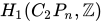
    Consider the braid group B n {\displaystyle B_{n}} {\displaystyle B_{n}} to be the mapping class group of a disc with n marked points, P n {\displaystyle P_{n}} {\displaystyle P_{n}}. The Lawrence–Krammer representation is defined as the action of B n {\displaystyle B_{n}} {\displaystyle B_{n}} on the homology of a certain covering space of the configuration space C 2 P n {\displaystyle C_{2}P_{n}} {\displaystyle C_{2}P_{n}}. Specifically, the first integral homology group of C 2 P n {\displaystyle C_{2}P_{n}} {\displaystyle C_{2}P_{n}} is isomorphic to Z n + 1 {\displaystyle \mathbb {Z} ^{n+1}} {\displaystyle \mathbb {Z} ^{n+1}}, and the subgroup of H 1 ( C 2 P n , Z ) {\displaystyle H_{1}(C_{2}P_{n},\mathbb {Z} )} {\displaystyle H_{1}(C_{2}P_{n},\mathbb {Z} )} invariant under the action of B n {\displaystyle B_{n}} {\displaystyle B_{n}} is primitive, free abelian, and of rank 2. Generators for this invariant subgroup are denoted by q , t {\displaystyle q,t} {\displaystyle q,t}.

    The covering space of C 2 P n {\displaystyle C_{2}P_{n}} {\displaystyle C_{2}P_{n}} corresponding to the kernel of the projection map

    π 1 ( C 2 P n ) Z 2 q , t {\displaystyle \pi _{1}(C_{2}P_{n})\to \mathbb {Z} ^{2}\langle q,t\rangle } {\displaystyle \pi _{1}(C_{2}P_{n})\to \mathbb {Z} ^{2}\langle q,t\rangle }

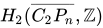
    is called the Lawrence–Krammer cover and is denoted C 2 P n ¯ {\displaystyle {\overline {C_{2}P_{n}}}} {\displaystyle {\overline {C_{2}P_{n}}}}. Diffeomorphisms of P n {\displaystyle P_{n}} {\displaystyle P_{n}} act on P n {\displaystyle P_{n}} {\displaystyle P_{n}}, thus also on C 2 P n {\displaystyle C_{2}P_{n}} {\displaystyle C_{2}P_{n}}, moreover they lift uniquely to diffeomorphisms of C 2 P n ¯ {\displaystyle {\overline {C_{2}P_{n}}}} {\displaystyle {\overline {C_{2}P_{n}}}} which restrict to the identity on the co-dimension two boundary stratum (where both points are on the boundary circle). The action of B n {\displaystyle B_{n}} {\displaystyle B_{n}} on

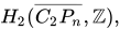
    H 2 ( C 2 P n ¯ , Z ) , {\displaystyle H_{2}({\overline {C_{2}P_{n}}},\mathbb {Z} ),} {\displaystyle H_{2}({\overline {C_{2}P_{n}}},\mathbb {Z} ),}

    thought of as a

    Z t ± , q ± {\displaystyle \mathbb {Z} \langle t^{\pm },q^{\pm }\rangle } {\displaystyle \mathbb {Z} \langle t^{\pm },q^{\pm }\rangle }-module,

    is the Lawrence–Krammer representation. The group H 2 ( C 2 P n ¯ , Z ) {\displaystyle H_{2}({\overline {C_{2}P_{n}}},\mathbb {Z} )} {\displaystyle H_{2}({\overline {C_{2}P_{n}}},\mathbb {Z} )} is known to be a free Z t ± , q ± {\displaystyle \mathbb {Z} \langle t^{\pm },q^{\pm }\rangle } {\displaystyle \mathbb {Z} \langle t^{\pm },q^{\pm }\rangle }-module, of rank n ( n 1 ) / 2 {\displaystyle n(n-1)/2} {\displaystyle n(n-1)/2}.
    Matrices

    Using Bigelow’s conventions for the Lawrence–Krammer representation, generators for the group H 2 ( C 2 P n ¯ , Z ) {\displaystyle H_{2}({\overline {C_{2}P_{n}}},\mathbb {Z} )} {\displaystyle H_{2}({\overline {C_{2}P_{n}}},\mathbb {Z} )} are denoted v j , k {\displaystyle v_{j,k}} {\displaystyle v_{j,k}} for 1 j < k n {\displaystyle 1\leq j<k\leq n} {\displaystyle 1\leq j<k\leq n}. Letting σ i {\displaystyle \sigma _{i}} {\displaystyle \sigma _{i}} denote the standard Artin generators of the braid group, we obtain the expression:
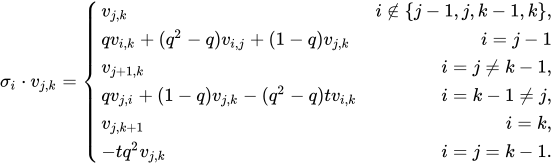
    σ i v j , k = { v j , k i { j 1 , j , k 1 , k } , q v i , k + ( q 2 q ) v i , j + ( 1 q ) v j , k i = j 1 v j + 1 , k i = j k 1 , q v j , i + ( 1 q ) v j , k ( q 2 q ) t v i , k i = k 1 j , v j , k + 1 i = k , t q 2 v j , k i = j = k 1. {\displaystyle \sigma _{i}\cdot v_{j,k}=\left\{{\begin{array}{lr}v_{j,k}&i\notin \{j-1,j,k-1,k\},\\qv_{i,k}+(q^{2}-q)v_{i,j}+(1-q)v_{j,k}&i=j-1\\v_{j+1,k}&i=j\neq k-1,\\qv_{j,i}+(1-q)v_{j,k}-(q^{2}-q)tv_{i,k}&i=k-1\neq j,\\v_{j,k+1}&i=k,\\-tq^{2}v_{j,k}&i=j=k-1.\end{array}}\right.} {\displaystyle \sigma _{i}\cdot v_{j,k}=\left\{{\begin{array}{lr}v_{j,k}&i\notin \{j-1,j,k-1,k\},\\qv_{i,k}+(q^{2}-q)v_{i,j}+(1-q)v_{j,k}&i=j-1\\v_{j+1,k}&i=j\neq k-1,\\qv_{j,i}+(1-q)v_{j,k}-(q^{2}-q)tv_{i,k}&i=k-1\neq j,\\v_{j,k+1}&i=k,\\-tq^{2}v_{j,k}&i=j=k-1.\end{array}}\right.}

    Faithfulness

    Stephen Bigelow and Daan Krammer have given independent proofs that the Lawrence–Krammer representation is faithful.

    Geometry

    The Lawrence–Krammer representation preserves a non-degenerate sesquilinear form which is known to be negative-definite Hermitian provided q , t {\displaystyle q,t} {\displaystyle q,t} are specialized to suitable unit complex numbers (q near 1 and t near i). Thus the braid group is a subgroup of the unitary group of square matrices of size n ( n 1 ) / 2 {\displaystyle n(n-1)/2} {\displaystyle n(n-1)/2}. Recently[2] it has been shown that the image of the Lawrence–Krammer representation is a dense subgroup of the unitary group in this case.

    The sesquilinear form has the explicit description:
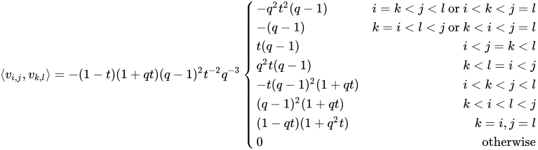
    v i , j , v k , l = ( 1 t ) ( 1 + q t ) ( q 1 ) 2 t 2 q 3 { q 2 t 2 ( q 1 ) i = k < j < l  or  i < k < j = l ( q 1 ) k = i < l < j  or  k < i < j = l t ( q 1 ) i < j = k < l q 2 t ( q 1 ) k < l = i < j t ( q 1 ) 2 ( 1 + q t ) i < k < j < l ( q 1 ) 2 ( 1 + q t ) k < i < l < j ( 1 q t ) ( 1 + q 2 t ) k = i , j = l 0 otherwise {\displaystyle \langle v_{i,j},v_{k,l}\rangle =-(1-t)(1+qt)(q-1)^{2}t^{-2}q^{-3}\left\{{\begin{array}{lr}-q^{2}t^{2}(q-1)&i=k<j<l{\text{ or }}i<k<j=l\\-(q-1)&k=i<l<j{\text{ or }}k<i<j=l\\t(q-1)&i<j=k<l\\q^{2}t(q-1)&k<l=i<j\\-t(q-1)^{2}(1+qt)&i<k<j<l\\(q-1)^{2}(1+qt)&k<i<l<j\\(1-qt)(1+q^{2}t)&k=i,j=l\\0&{\text{otherwise}}\\\end{array}}\right.} {\displaystyle \langle v_{i,j},v_{k,l}\rangle =-(1-t)(1+qt)(q-1)^{2}t^{-2}q^{-3}\left\{{\begin{array}{lr}-q^{2}t^{2}(q-1)&i=k<j<l{\text{ or }}i<k<j=l\\-(q-1)&k=i<l<j{\text{ or }}k<i<j=l\\t(q-1)&i<j=k<l\\q^{2}t(q-1)&k<l=i<j\\-t(q-1)^{2}(1+qt)&i<k<j<l\\(q-1)^{2}(1+qt)&k<i<l<j\\(1-qt)(1+q^{2}t)&k=i,j=l\\0&{\text{otherwise}}\\\end{array}}\right.}

    References

    1. Bigelow, Stephen (2003), “The Lawrence–Krammer representation”, Topology and geometry of manifolds, Proc. Sympos. Pure Math., vol. 71, Providence, RI: Amer. Math. Soc., pp. 51–68, MR 2024629
    2. Budney, Ryan (2005), “On the image of the Lawrence–Krammer representation”, Journal of Knot Theory and Its Ramifications, 14 (6): 773–789, arXiv:math/0202246, doi:10.1142/S0218216505004044, MR 2172897, S2CID 14196563

    Further reading


    This article is adapted from “Lawrence–Krammer representation” on Wikipedia, written by its contributors, and used under CC BY-SA 4.0. Text on this page is available under the same licence. Source snapshot: Wikipedia via Kiwix, 2026-07-20.
  • Lapp knot

    Lapp knot
    Lapp knot
    Names Lapp knot, Lap knot, Lap bend, Lapp bend, quick hitch
    Category Bend
    Category 2 Loop
    Origin Ancient
    Related sheet bend, bowline, cowboy bowline, Eskimo bowline
    Releasing Non-jamming
    Typical use Joining two lines, loop, binding knot
    ABoK #1224

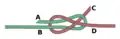
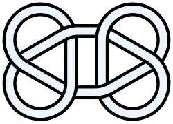
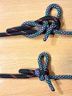
    The Lapp knot is a type of bend. It has the same structure as the sheet bend, but the opposite ends are loaded. The slipped Lapp bend (among arbourists known as quick hitch) is also an exploding knot, which means that when pulling the quick release end it falls completely apart without further entanglement. It is as strong as or even stronger than the sheet bend,[1] though much less common.

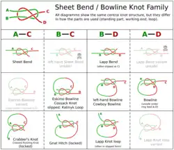
    The Lapp knot is closely related to the sheet bend, the bowline and the Eskimo bowline. They all share the same core structure, but differ in how the four ends are loaded.
    The Lapp knot was sometimes called ‘false sheet bend’,[2] which might explain its low popularity.

    Lapp bend

    Lapp knot
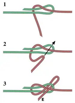
    Steps to tie a (slipped) Lapp bend.
    Lapp knot
    Bends and loops directly related to the sheet bend and bowline

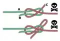
    A way to tie the knot is shown in the image to the left. The orientation of the green bight is important: Its working end should end up on the same side as the red lines slip bight, or as the red working end when tying the non-slip version (A & C). If they end up on opposite sides (B & C), the resulting knot is much weaker and tends to slip, because then the two standing parts lose some of their binding force due to mutual friction before they can clamp down the loose ends. (The same is true for the bowline.)

    The non-slipped Lapp bend (like the bowline) does not jam and can be untied easily even after being loaded. The slipped version unties even easier with a firm tug on the end E (quick release).

    • The non-slipped version of the Lapp bend.
      The non-slipped version of the Lapp bend.
    • The Lapp Bend's unsafe sibling with working ends on opposite sides.
      The Lapp Bend’s unsafe sibling with working ends on opposite sides.

    Lapp knot as loop

    Lapp knot
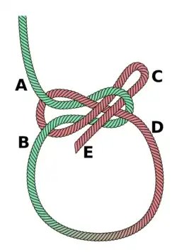
    The Lapp Knot as loop.

    The Lapp knot can be tied as a loop knot, in which case A becomes the standing part in the loop, B and D the two strands of the loop, and C the free end. It is also a secure loop if B is the standing part rather than A, though this variation is insecure under ring loading as it mimics the weaker version of the Lapp bend.

    The knot loses some of its adjustability after the standing part has been loaded. If the knot isn’t tightened properly before loading, or A and B are pulled apart, it might capsize into a Mooring hitch. The knot can also be tied by first tying a Mooring hitch, then adjusting it to the desired size, then pulling the slipped end away from the loop.

    If D is the standing part, rather than A, the result is commonly known as the Eskimo bowline.

    Lapp knot as (adjustable) binding knot

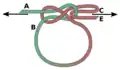
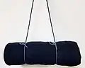
    The slipped Lapp knot can also be used as a binding knot for bundles or rolls (or a bathrobe). Its advantage over the reef knot is that the finished knot can be tightened by pulling the slip loop and end (C+E) and the working end A in opposite directions, or loosened by pulling B instead of A. When releasing C+E, it pulls tight again. Pulling only end E dissolves it completely.

    • Tightening the Lapp knot loop.
      Tightening the Lapp knot loop.
    • Lapp knot used as quick-release binding knot (to tie up a rolled jacket) and as loop (to hang it up by the standing part).
      Lapp knot used as quick-release binding knot (to tie up a rolled jacket) and as loop (to hang it up by the standing part).

    History

    The knot is documented since 1892 under various names (false weaver’s bend, false sheet bend, English Bowline, Girdle Knot), and was used by various native cultures (America, Lapland, Africa, Australia).[3] The name Lap(p) knot stems from it having been used in Lapland to tie reindeer to a sled and for lanyards. The slipped Lapp knot is also shown in The Ashley Book of Knots as #1224, a nameless decorative bathrobe cord knot.

    Alternatives

    As a bend:

    As a loop:

    As a binding knot:

    • The reef knot is much more common, but not adjustable.
    • A jamming knot (a rolling hitch tied around the other end) can also be used as an adjustable binding knot. Using a Farrimond friction hitch (tied like the hitch as the Farrimond friction hitch is bidirectional) maintains the exploding property of the Lapp knot.
    • The constrictor knot can be tightened much more tightly, but needs more rope and unties less easily.
    • Other binding knots

    References

    1. Compton, Nic (2013). The Knot Bible. Adlard Coles Nautical. p. 83. ISBN 978-1-4081-5476-2.
    2. Budworth, Geoffrey (1997). The Complete Book of Knots. The Lyons Press. p. 34. ISBN 1-55821-632-4.
    3. Knotting Matters 52, International Guild of Knot Tyers, April 1996

    External links


    This article is adapted from “Lapp knot” on Wikipedia, written by its contributors, and used under CC BY-SA 4.0. Text on this page is available under the same licence. Source snapshot: Wikipedia via Kiwix, 2026-07-20.
  • Lamp cord trick

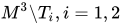
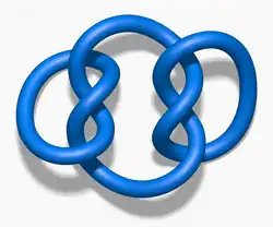
    In topology, a branch of mathematics, and specifically knot theory, the lamp cord trick is an observation that two certain spaces are homeomorphic, even if one of the components is knotted. The spaces are M 3 T i , i = 1 , 2 {\displaystyle M^{3}\backslash T_{i},i=1,2} {\displaystyle M^{3}\backslash T_{i},i=1,2}, where M 3 {\displaystyle M^{3}} {\displaystyle M^{3}} is a hollow ball homeomorphic to S 2 × [ 0 , 1 ] {\displaystyle S^{2}\times [0,1]} {\displaystyle S^{2}\times [0,1]} and T i {\displaystyle T_{i}} {\displaystyle T_{i}} a tube connecting the boundary components of M 3 {\displaystyle M^{3}} {\displaystyle M^{3}}. The name comes from R. H. Bing’s book “The Geometric Topology of 3-manifolds”.[1]

    References

    1. Bing, R. H. (31 December 1983). The Geometric Topology of 3-manifolds. ISBN 9780821810408.
    • Lucien Grillet, La Conjecture de Smith en faible régularité.


    This article is adapted from “Lamp cord trick” on Wikipedia, written by its contributors, and used under CC BY-SA 4.0. Text on this page is available under the same licence. Source snapshot: Wikipedia via Kiwix, 2026-07-20.

  • L10a140 link

    L10a140
    L10a140 link
    Braid length 10
    Braid no. 3
    Crossing no. 10
    Hyperbolic volume 12.27627758
    Conway notation [.3:30]
    Thistlethwaite L10a140
    Other
    alternating

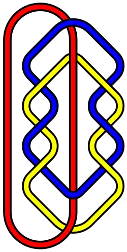
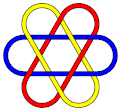
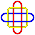
    In the mathematical theory of knots, L10a140 is the name in the Thistlethwaite link table of a link of three loops, which has ten crossings between the loops when presented in its simplest visual form.[1] It is of interest because it is presumably the simplest link which possesses the Brunnian property — a link of connected components that, when one component is removed, becomes entirely unconnected[2] — other than the six-crossing Borromean rings.[3]

    In other words, no two loops are directly linked with each other, but all three are collectively interlinked, so removing any loop frees the other two. In the image in the infobox at right, the red loop is not interlinked with either the blue or the yellow loops, and if the red loop is removed, then the blue and yellow loops can also be disentangled from each other without cutting either one.

    According to work by Slavik V. Jablan, the L10a140 link can be seen as the second in an infinite series of Brunnian links beginning with the Borromean rings. So if the blue and yellow loops have only one twist along each side, the resulting configuration is the Borromean rings; if the blue and yellow loops have three twists along each side, the resulting configuration is the L10a140 link; if the blue and yellow loops have five twists along each side, the resulting configuration is a three-loop link with 14 overall crossings, etc. etc.[4]

    Invariants

    The multivariable Alexander polynomial for the L10a140 link is

    Δ ( u , v , w ) = ( u 1 ) ( v 1 ) ( w 1 ) ( v w + 1 ) 2 v w u v w , {\displaystyle \Delta (u,v,w)={\frac {(u-1)(v-1)(w-1)(vw+1)^{2}}{vw{\sqrt {uvw}}}},\,} {\displaystyle \Delta (u,v,w)={\frac {(u-1)(v-1)(w-1)(vw+1)^{2}}{vw{\sqrt {uvw}}}},\,}

    the Conway polynomial is

    ( z ) = 4 z 4 + 4 z 6 + z 8 , {\displaystyle \nabla (z)=4z^{4}+4z^{6}+z^{8},\,} {\displaystyle \nabla (z)=4z^{4}+4z^{6}+z^{8},\,}

    the Jones polynomial factors nicely as

    V ( t ) = t 5 + 3 t 4 5 t 3 + 8 t 2 9 t + 12 9 t 1 + 8 t 2 5 t 3 + 3 t 4 t 5 = 1 t 5 ( t 5 2 t 4 + t 3 2 t 2 + t 1 ) ( t 5 t 4 + 2 t 3 t 2 + 2 t 1 ) = w ( t ) w ( 1 / t ) , {\displaystyle {\begin{aligned}V(t)&=-t^{5}+3t^{4}-5t^{3}+8t^{2}-9t+12-9t^{-1}+8t^{-2}-5t^{-3}+3t^{-4}-t^{-5}\\[8pt]&=-{\frac {1}{t^{5}}}\left(t^{5}-2t^{4}+t^{3}-2t^{2}+t-1\right)\left(t^{5}-t^{4}+2t^{3}-t^{2}+2t-1\right)\\[8pt]&=w(t)w(1/t),\,\end{aligned}}} {\displaystyle {\begin{aligned}V(t)&=-t^{5}+3t^{4}-5t^{3}+8t^{2}-9t+12-9t^{-1}+8t^{-2}-5t^{-3}+3t^{-4}-t^{-5}\\[8pt]&=-{\frac {1}{t^{5}}}\left(t^{5}-2t^{4}+t^{3}-2t^{2}+t-1\right)\left(t^{5}-t^{4}+2t^{3}-t^{2}+2t-1\right)\\[8pt]&=w(t)w(1/t),\,\end{aligned}}}

    where w ( t ) = t 5 2 t 4 + t 3 2 t 2 + t 1. {\displaystyle w(t)=t^{5}-2t^{4}+t^{3}-2t^{2}+t-1.} {\displaystyle w(t)=t^{5}-2t^{4}+t^{3}-2t^{2}+t-1.} (Notice that w ( t ) {\displaystyle w(t)} {\displaystyle w(t)} is essentially the Jones polynomial for the Whitehead link.)

    The HOMFLY polynomial is

    P ( α , z ) = z 2 α 2 4 z 2 α 2 4 z 4 α 2 z 6 α 2 2 z 2 + 8 z 2 + 12 z 4 + 6 z 6 + z 8 + z 2 α 2 4 z 2 α 2 4 z 4 α 2 z 6 α 2 , {\displaystyle P(\alpha ,z)=z^{-2}\alpha ^{-2}-4z^{2}\alpha ^{-2}-4z^{4}\alpha ^{-2}-z^{6}\alpha ^{-2}-2z^{-2}+8z^{2}+12z^{4}+6z^{6}+z^{8}+z^{-2}\alpha ^{2}-4z^{2}\alpha ^{2}-4z^{4}\alpha ^{2}-z^{6}\alpha ^{2},\,} {\displaystyle P(\alpha ,z)=z^{-2}\alpha ^{-2}-4z^{2}\alpha ^{-2}-4z^{4}\alpha ^{-2}-z^{6}\alpha ^{-2}-2z^{-2}+8z^{2}+12z^{4}+6z^{6}+z^{8}+z^{-2}\alpha ^{2}-4z^{2}\alpha ^{2}-4z^{4}\alpha ^{2}-z^{6}\alpha ^{2},\,}

    and the Kauffman polynomial is

    F ( a , z ) = 1 + 2 z 2 + a 2 z 2 + a 2 z 2 2 a 1 z 1 a z 1 20 z 2 + 2 a 4 z 2 8 a 2 z 2 8 a 2 z 2 + 2 a 4 z 4 + 2 a 4 z 2 2 a 5 z 3 + 4 a 3 z 3 + 6 a 1 z 3 + 6 a z 3 + 4 a 3 z 3 2 a 5 z 3 + 42 z 4 7 a 4 z 4 + 14 a 2 z 4 + 14 a 2 z 4 7 a 4 z 4 + a 5 z 5 9 a 3 z 5 2 a 1 z 5 2 a z 5 9 a 3 z 5 + a 5 z 5 28 z 6 + 3 a 4 z 6 11 a 2 z 6 11 a 2 z 6 + 3 a 4 z 6 + 4 a 3 z 7 2 a 1 z 7 2 a z 7 + 4 a 3 z 7 + 8 z 8 + 4 a 2 z 8 + 4 a 2 z 8 + 2 a 1 z 9 + 2 a z 9 . {\displaystyle {\begin{aligned}F(a,z)&=1+2z^{-2}+a^{-2}z^{-2}+a^{2}z^{-2}-2a^{-1}z^{-1}-az^{-1}-20z^{2}+2a^{-4}z^{2}\\[6pt]&{}-8a^{-2}z^{2}-8a^{2}z^{2}+2a^{4}z^{4}+2a^{4}z^{2}-2a^{-5}z^{3}+4a^{-3}z^{3}+6a^{-1}z^{3}\\[6pt]&{}+6az^{3}+4a^{3}z^{3}-2a^{5}z^{3}+42z^{4}-7a^{-4}z^{4}+14a^{-2}z^{4}\\[6pt]&{}+14a^{2}z^{4}-7a^{4}z^{4}+a^{-5}z^{5}-9a^{-3}z^{5}-2a^{-1}z^{5}-2az^{5}-9a^{3}z^{5}\\[6pt]&{}+a^{5}z^{5}-28z^{6}+3a^{-4}z^{6}-11a^{-2}z^{6}-11a^{2}z^{6}+3a^{4}z^{6}+4a^{-3}z^{7}\\[6pt]&{}-2a^{-1}z^{7}-2az^{7}+4a^{3}z^{7}+8z^{8}+4a^{-2}z^{8}+4a^{2}z^{8}+2a^{-1}z^{9}+2az^{9}.\end{aligned}}} {\displaystyle {\begin{aligned}F(a,z)&=1+2z^{-2}+a^{-2}z^{-2}+a^{2}z^{-2}-2a^{-1}z^{-1}-az^{-1}-20z^{2}+2a^{-4}z^{2}\\[6pt]&{}-8a^{-2}z^{2}-8a^{2}z^{2}+2a^{4}z^{4}+2a^{4}z^{2}-2a^{-5}z^{3}+4a^{-3}z^{3}+6a^{-1}z^{3}\\[6pt]&{}+6az^{3}+4a^{3}z^{3}-2a^{5}z^{3}+42z^{4}-7a^{-4}z^{4}+14a^{-2}z^{4}\\[6pt]&{}+14a^{2}z^{4}-7a^{4}z^{4}+a^{-5}z^{5}-9a^{-3}z^{5}-2a^{-1}z^{5}-2az^{5}-9a^{3}z^{5}\\[6pt]&{}+a^{5}z^{5}-28z^{6}+3a^{-4}z^{6}-11a^{-2}z^{6}-11a^{2}z^{6}+3a^{4}z^{6}+4a^{-3}z^{7}\\[6pt]&{}-2a^{-1}z^{7}-2az^{7}+4a^{3}z^{7}+8z^{8}+4a^{-2}z^{8}+4a^{2}z^{8}+2a^{-1}z^{9}+2az^{9}.\end{aligned}}}

    Pseudo-symmetric visual variants

    David Swart,[5] and independently Rick Mabry and Laura McCormick,[6] discovered alternative 12-crossing visual representations of the L10a140 link. In these depictions, the link no longer has strictly alternating crossings (as it does in its simplest 10-crossing form), but there is greater superficial symmetry.

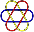
    So the leftmost image below shows a 12-crossing link (distinct from both the Borromean rings and the L10a140 link) with six-fold rotational symmetry. The center image shows a similar-looking depiction of the L10a140 link (but without true rotational symmetry). Similarly, the rightmost image shows a depiction of the L10a140 link with superficial fourfold symmetry.

    • Fully symmetrical 12-crossing Brunnian link (L12a1882)
      Fully symmetrical 12-crossing Brunnian link (L12a1882)
    • L10a140 in pseudo 6-symmetric form
      L10a140 in pseudo 6-symmetric form
    • L10a140 in pseudo 4-symmetric form
      L10a140 in pseudo 4-symmetric form

    References

    1. L10a140“, The Knot Atlas.
    2. Adams, Colin C. (1994). The Knot Book. American Mathematical Society. p. 22. ISBN 9780716723936.
    3. Bar-Natan, Dror (2010-08-16). “All Brunnians, Maybe“, Academic Pensieve.
    4. Jablan, Slavik V., Are Borromean Links So Rare?, Forma 14 (1999), 269277. Online at the electronic journal Vismath. L10a140 is depicted in the middle figure of the top image.
    5. Dror Bar-Natan (2010-08-14). “A Link from David Swart“, [Academic Pensieve].
    6. Swart, David (April 2011). “It is what it is”. Math Horizons. 18 (4).

    External links


    This article is adapted from “L10a140 link” on Wikipedia, written by its contributors, and used under CC BY-SA 4.0. Text on this page is available under the same licence. Source snapshot: Wikipedia via Kiwix, 2026-07-20.

  • Korean knots

    Korean knots, also known as maedeup (매듭), is a traditional Korean handicraft. The current form dates back to the Three Kingdom periods.

    Korean knotting uses a unique braiding technique.[1] Korean knotting is derived from the ancient practice of using knots for practical purposes; e.g. in fishing nets, agricultural tools, stone knives and axes.[1][2]

    Traditionally, the knots were used primarily to hold hunting tools around the waist and their usage was initially limited to royal families, spreading later to common people. Today, modern Korean artists are using the traditional knots in their works, such as accessories, jewelry and home interior decorations.[1]

    Design

    Korean knots are tighter than both then Chinese knots and Japanese knots; maedeup is also more three-dimensional than the other East Asian knots.[1][2][3] Maedeup also has a longer tassel than the Chinese knots.[4] Another main difference between Chinese and Korean knots is color and type of cord used.[4]

    The finished knot has the same shape at the front and at the back, has bilateral symmetry.[2][5] It can be made using one or two threads.

    History of Korean Knots

    Prehistory

    In Neolithic times, Korean knots were used solely for practical purposes; they were tied around the waist and used to carry stone-axes, swords, and other tools used for hunting and food.[1][2][5][6]

    Tools that was used for sewing and knotting such as Garak-Bakwi, was excavated throughout various regions of Korea. Garak-Bakwi from the Stone Age exhibit holes where thread was looped through and then knotted. Similar evidence is found in relics of the Bronze Age. The knots were strengthened by twisting or weaving multiple strings.

    Three Kingdoms of Korea (4th century – 668 CE)

    The oldest record of maedup can be found in Goguryeo painting which dates from 357 AD.[5] During the period of the Three Kingdoms of Korea, people began to see aesthetic value in knots. The Korean knot which used to be only for practical use developed in a form of decorative art.[6]

    People started to use them as decorations on clothes, swords, and more.[7] The Samguk Sagi, the oldest extant record of Korean history, describes knot usage in everyday life during the Silla dynasty, noting rulers enjoyed using knots to adorn horses.[7] It is also told that there was specific dress code for the nobles about designs of clothes, which includes knots during the King Heong-deok of Silla.

    Period of the Goryeo dynasty (918-1392)

    Formal knots are depicted in buddhist murals and paintings in the Goryeo dynasty.[1][2] During this period, knots were widely used as ornaments in accessories and for art.

    For example, In the Portrait of Lee Je-Hyeon, who was a civil vassal(Munshin) shows that the decoration of knots. Also, the specific style can be found in a blue-green celadon made during the Goryeo Dynasty.

    Period of Joseon dynasty (1392-1910)

    During the Joseon dynasty, knots became more diverse and elaborate. They were a symbol of high social status and it was considered a sign of dignity and prestige in the royal palace.[1] They were used to decorate traditional instruments and clothes, especially women’s garments and jewelry (e.g. necklace, pendants, and earrings).[3] The Joseon rulers hired their own knot-makers to decorate the palace and jewelry for the noble family.[1][3]

    The particular crocheting skill called Dahoe and Mangsu was used when making garments for royal members, and there was special artisan in royal palace that specialized in such craft. In early era, the Dahoe artisan and Maedeup artisans were differentiated, but later the job has been overlapped, as Dahoejang, a Dahoe artisan is doing the both art.[8]

    Korea under Japanese Rule (1910-1945)

    Demand for knots were so high among Koreans that knots became commercialized. But demand decreased after the Japanese enacted policies designed to obliterate Korean culture and a surge of Western culture into the Korean peninsula shifted traditions. They became rarely seen in public.

    Types of Korean knots

    There are more than 30 basic types of knots.[2] Some sources state that there is 38 basic knots.[5] But there are vast numbers of variations and regional version on these basic types. Some of the most common knots include:

    • Dalgi knot – this knot resembles a strawberry.
    • Dorae knot – the most basic form of knot,[1] it is used to connect knots and to fix or finish a knot.
    • Guidorae knot – there are many different names that describe this type of knot, but is normally called the Guidorae. This knot tends not to be fixed.
    • Gukwa knot (also written as “gukhwa“) – chrysanthemum knot; when tied in plum and mauve threads, it apparently represents autumn and eternity.[9][10] It is similar to the Chinese Pan Chang knot in construction.[9]
    • Maehwa knot – this knot resembles a Japanese apricot flower;[1] and it is used for baby clothes and Norigae, Korean traditional ornaments worn by women.
    • Nabi knot – butterfly knot.[10]
    • Saengjok knot – Ginger knot.[9]

    Usage of Korean knots

    Knots of diverse colors were used as belts, identity tags, and as a decorative element on instruments. In the ruling palaces, knots were used to signify dignity and prestige. For religious purposes knots decorated Buddhist ornaments.

    The most common use of knots was in Norigae, traditional Korean ornaments worn by women to decorate clothing. Norigae were used by all ages and social statuses to emphasize the beauty of Korean traditional costume, as well as decorate pockets carried separately. Though these knots were used across all social statuses, there were also cases when only specific people were allowed to use them. For example, only high government officials were allowed to use knots for decorating fans.

    Korean Knots in modern Korea

    After the establishment of a cultural industry bureau in South Korea in 1994, the use of knots modern life increased, especially in cultural products. Korean knots were also used in the designs of non-Korean artists, usually in forms of the Garackji knot (a basic knot used to fill space and give a classical touch) and the Mangsa knot (used on pouches for jewelry).

    As a National Intangible Cultural Heritage of Korea

    The skill of Maedeupt craft is designated as a National Heritage of South Korea in 1968.[11] The special skill is succeed by lineage of artisans.

    The first Maedueptjang who is designated as National Heritage was Jeong Yun-su, who was designated as master in 1968, who was succeeded by Choi Eun-sun in 1974. The skill is still being preserved by many succeeding artisans nowadays[12]

    References

    1. 1 2 3 4 5 6 7 8 9 10 “Knot dying out: traditional craft of 𝘮𝘢𝘦𝘥𝘦𝘶𝘱”. Korea.net. Retrieved 2021-04-09.
    2. 1 2 3 4 5 6 “KOREA webzine _ Crafts”. Korean Culture and Information Service (in Korean). Retrieved 2021-04-13.
    3. 1 2 3 “Why Knot in Life?”. The Korea Times. 2007-05-01. Retrieved 2021-04-13.
    4. 1 2 Chen, Lydia (2014). The complete book of chinese knotting: a compendium of techniques and variations. New York: Tuttle Publishing. p. 16. ISBN 978-1-4629-1645-0. OCLC 904404949.
    5. 1 2 3 4 Meverden, Becky (2009). Elegant knotted jewelry. Cincinnati, OH: Krause Pub. ISBN 978-1-4402-2364-8. OCLC 767499934.
    6. 1 2 Victoria and Albert Museum, Digital Media (2014-01-23). “Maedŭp: The Craft of Knotting”. www.vam.ac.uk. Retrieved 2021-04-13.
    7. 1 2 Lee, Eun-Hyung (November 2009). “Historial Review of Korean Traditional Baeja, and an Exploration of its Modernization”. Journal of the Korean Society of Costume. 59 (9): 3 via KCI.
    8. Seol, Ji-Hee (2021). “A Study on the Roles of Daheojang and Maedeupjang in the Joseon Dynasty”. Korean Journal of Heritage: History and Science. 54 (3).
    9. 1 2 3 Philpott, Lindsey (2013). The Ultimate Book of Decorative Knots. New York: Skyhorse Publishing, Inc. p. 500. ISBN 978-1-62873-415-7. OCLC 855969176.
    10. 1 2 Kim, Bo-Young; Geum, Key-Sook (2010). “A Study on the Formative Aesthetics and Modern Application of Traditional Korean Knots [Abstract]. Journal of the Korean Society of Costume. 60 (10): 1–15. ISSN 1229-6880.
    11. “국가유산 종목별 검색”.
    12. “국가유산진흥원”. www.kh.or.kr (in Korean). Retrieved 2025-03-07.
    1. Lee Jong Kyu, “Study of Fashion design using Korean Traditional Knots” (한국전통매듭을 응용한 패션 디자인 연구), Master’s Thesis. Sookmyung Women’s College. (2009)
    2. Lim Young Ju, “Study of Korean Traditional Knots”(한국 전통 매듭에 관한 연구), Doctor’s Thesis. Won Kwang University. (2002)
    3. Kim Johnson Young, “Study of accessory design using Korean Traditional knots (한국전통매듭을 응용한 장신구 디자인 연구), Master’s Thesis. SungKyunkwan University. (2005)

    This article is adapted from “Korean knots” on Wikipedia, written by its contributors, and used under CC BY-SA 4.0. Text on this page is available under the same licence. Source snapshot: Wikipedia via Kiwix, 2026-07-20.

  • Knute hitch

    Knute hitch
    Knute hitch
    Category Hitch
    Related Marlinespike hitch
    Releasing Non-jamming
    Typical use Attaching a lanyard to a tool

    The Knute hitch is used to attach a lanyard of small stuff to a marlingspike or other tool. Rigger Brion Toss named the hitch after his favourite marlingspike of the same name,[1] although the hitch is likely much older.[2]

    Tying

    The lanyard line should be just small enough to fit doubled through the lanyard hole in the tool. This is done, forming a protruding bight. The end, with a figure-eight knot stopper, is placed through the bight but not fully pulled through. Finally, the bight is withdrawn, jamming the bight and line end in the hole. To release, pull on the end and remove it from the bight.

    See also

    References

    1. Toss, Brion (1992). The Rigger’s Locker – Tools and Techniques for Modern and Traditional Rigging. International Marine. p. 105.
    2. Budworth, Geoffrey (1999). The Ultimate Encyclopedia of Knots & Ropework. London: Hermes House. p. 102.

    External links


    This article is adapted from “Knute hitch” on Wikipedia, written by its contributors, and used under CC BY-SA 4.0. Text on this page is available under the same licence. Source snapshot: Wikipedia via Kiwix, 2026-07-20.

  • Knotted-pile carpet

    Knotted-pile carpet
    Ghiordes knot
    Knotted-pile carpet
    Senneh knot
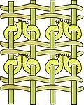
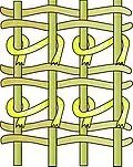
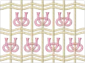
    The yellow yarn is the pile and the horizontal and vertical yarns are the warp and the weft.

    A knotted-pile carpet is a carpet containing raised surfaces, or piles, from the cut off ends of knots woven between the warp and weft. The Ghiordes/Turkish knot and the Senneh/Persian knot, typical of Anatolian carpets and Persian carpets, are the two primary knots.[1] A flat or tapestry woven carpet, without pile, is a kilim. A pile carpet is influenced by width and number of warp and weft, pile height, knots used, and knot density.

    “The structural weft threads alternate with supplementary weft that rises from the surface of the weave at a perpendicular angle. This supplementary weft is attached to the warp by one of three knots… to form the pile or nap of the carpet.”[2] Knots are tied in rows, one to each pair of warp threads, which may then be pushed down to make the rug more solid: “the interwoven warp and weft threads form the carpet’s foundation, and the design comes from the rows of knots.”[3] “In the knotted-pile…the arrangement of rows of weft is the dominant consideration.”[4]

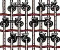
    Diagonal, or offset, knotting has knots in successive rows occupy alternate pairs of warps. This feature allows for changes from one half knot to the next, and creates diagonal pattern lines at different angles. It is sometimes found in Kurdish or Turkmen rugs, particularly in Yomuds. It is mostly tied symmetrically.[5]

    Ghiordes

    Knotted-pile carpet
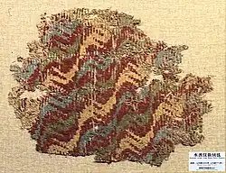
    Knotted carpet with colorful wave-like motifs from Yanghai (Subeshi culture) were dated to 700 BCE, and are now the oldest known knotted carpet in the world, before the 4th century BCE Pazyryk carpets. Turpan Museum.[6]
    Knotted-pile carpet
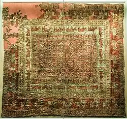
    Decorated knotted-pile carpet from Pazyryk-5. 4th century BCE.[7]

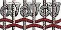
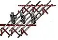
    The Ghiordes knot, symmetrical knot or Turkish knot is one of the two most-used knots employed in knotted-pile carpets. In the Ghiordes knot, the colored weft yarn passes over the two warp yarns, and is pulled through between them and then cut to form the pile. The Ghiordes knot has a symmetrical structure. The Ghiordes knot is the knot used in the oldest surviving pile carpets, the fragments found in Pazyryk kurgan burial mounds, in the Altai of Central Asia.[8] The Ghiordes knot is also used in Turkeywork textiles of the Early Modern period.[9]

    To tie a Ghiordes knot, the yarn is passed between two adjacent warps, brought back under one, wrapped around both forming a collar, then pulled through the center so that both ends emerge between the warps.[10] The Ghiordes knot uses two warps.

    Senneh

    Persian carpets are mainly woven with two different knots: the symmetrical Turkish or “Ghiordes” knot, also used in Turkey, the Caucasus, East Turkmenistan, and some Turkish and Kurdish areas of Iran; and the asymmetrical Persian, or Senneh knot, also used in India, Turkey, Pakistan, China, and Egypt. The term “Senneh knot” is somewhat misleading, as rugs are woven with symmetric knots in the town of Senneh.[10]

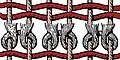
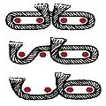
    The asymmetric knot is tied by wrapping the yarn around only one warp, then the thread is passed behind the adjacent warp so that it divides the two ends of the yarn. The Persian knot may open on the left or the right.[10] The Persian knot may be considered as using two warps, or only warp.

    The asymmetric knot allows the artist to produce more fluent, often curvilinear designs, while more bold, rectilinear designs may use the symmetric knot. As exemplified by Senneh rugs with their elaborate designs woven with asymmetric knots, the quality of the design depends more on the weaver’s skills, than on the type of knot which is used.[10]

    Jufti

    Another knot frequently used in Persian carpets is the Jufti knot, which is tied around four warps instead of two.[5][1] A serviceable carpet can be made with jufti knots, and jufti knots are sometimes used in large single-colour areas of a rug, for example in the field, to save on material. However, as carpets woven wholly or partly with the jufti knot need only half the amount of pile yarn compared to traditionally woven carpets, their pile is less resistant to wear, and these rugs do not last as long.[10]

    Other knots

    Another variant of knot is known from early Spanish rugs. The Spanish knot or single-warp knot, is tied around one single warp. Some of the rug fragments excavated by A. Stein in Turfan seem to be woven with a single knot. Single knot weavings are also known from Egyptian Coptic pile rugs.[11]

    Knot gallery

    • Turkish (symmetric) knot
      Turkish (symmetric) knot
    • Persian (asymmetric) knot, open to the right
      Persian (asymmetric) knot, open to the right
    • Variants of the "Jufti" knot woven around four warps
      Variants of the “Jufti” knot woven around four warps
    • Spanish knot or single-warp knot
      Spanish knot or single-warp knot
    • Diagonal, or offset, knotting
      Diagonal, or offset, knotting
    • Weaving with one warp depressed
      Weaving with one warp depressed
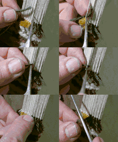
    • Knitting an asymmetric knot, open to the right, with a knitting hook similar to the Tabriz type
      Knitting an asymmetric knot, open to the right, with a knitting hook similar to the Tabriz type
    • Knotted-pile carpet

    See also

    • Pile weave

    References

    1. 1 2 Goswami, K.K.; ed. (2009). Advances in Carpet Manufacture, p.239. Woodhead Publishing in Textiles: Number 87 (The Textile Institute). ISBN 9781845695859. “The two most common types of knot used in an oriental carpet are the Persian knot and the Turkish knot.”
    2. Goswami (2009), p.220.
    3. Rosemary Troy Krill (2010). Early American Decorative Arts, 1620-1860: A Handbook for Interpreters, p.248. Rowman Altamira. ISBN 9780759119468.
    4. (1921). Tariff Information Surveys, p.15. U.S. Government Printing Office. [ISBN unspecified].
    5. 1 2 Eilland, Murray L. Jr.; Eilland, Murray III (1998). Oriental Rugs – A Complete Guide (revised ed.). London: Callmann & King Ltd.
    6. He, Zhang (2019). “Knotted Carpets from the Taklamakan: A Medium of Ideological and Aesthetic Exchange on the Silk Road, 700 BCE-700 CE” (PDF). The Silk Road. 17. Dated to as early as 700 BCE (Jia et al. 2009), the Yanghai carpet pieces are approximately three centuries older than the Pazyryk carpets (Rudenko 1970), making them the earliest knotted carpets found anywhere in the world.
    7. Pankova, Svetlana; Simpson, St John (1 January 2017). Scythians: warriors of ancient Siberia. p. 281.
    8. Conserved in the Hermitage Museum, St. Petersburg.
    9. “Turkeywork”. Getty Art & Architecture Thesaurus. Retrieved 16 May 2018.
    10. 1 2 3 4 5 Edwards, A. Cecil (1975). The Persian carpet: a survey of the carpet-weaving industry of Persia (Reprinted 1952 ed.). London: Duckworth. ISBN 978-0715602560.
    11. Eilland, Murray L. Jr.; Eilland, Murray III (1998). Oriental Rugs – A Complete Guide (revised ed.). London: Callmann & King Ltd. pp. 37–38. ISBN 978-0821225486.

    External links

    • Ghiordes knot” – Encyclopaedia Britannica. Accessed: June 26, 2020.

    This article is adapted from “Knotted-pile carpet” on Wikipedia, written by its contributors, and used under CC BY-SA 4.0. Text on this page is available under the same licence. Source snapshot: Wikipedia via Kiwix, 2026-07-20.
  • Knots in Washington

    Knots in Washington is an international conference on knot theory and its ramifications held twice a year since 1995. The main organizers are Józef Przytycki, Alexander Shumakovitch, Yongwu Rong and Valentina Harizanov, all of whom are at George Washington University.[1]

    This conference has become an important topological event in the Washington Metropolitan Area and regularly attracts well-known topologists from other areas of the US and from other countries.[2] For example, Knots in Washington XVIII, held in May 2004, was the first conference fully devoted to the Khovanov homology, with Mikhail Khovanov giving a series of talks and leading experts Dror Bar-Natan, Lev Rozansky, Oleg Viro, and Ciprian Manolescu giving plenary talks.[3] Knots in Washington XX was dedicated to the 60th birthday of Louis H. Kauffman.[4] Other related conferences include Knots in Poland (1995, 2003),[5] and Knots in Hellas in 1998, where Fields Medal winner Vaughan Jones spoke about his work on knot invariants.[6]

    Knots in Washington 50 will take place Dec 6th-8th, 2024 at the George Washington University with updated website: https://blogs.gwu.edu/ccas-knotsinwashington/

    References

    External links


    This article is adapted from “Knots in Washington” on Wikipedia, written by its contributors, and used under CC BY-SA 4.0. Text on this page is available under the same licence. Source snapshot: Wikipedia via Kiwix, 2026-07-20.