Blog

  • Knots Unravelled

    Knots Unravelled
    First edition

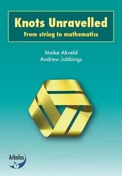
    Knots Unravelled: From String to Mathematics is a book on the mathematics of knots, intended for schoolchildren and other non-mathematicians. It was written by mathematician Meike Akveld and mathematics publisher Andrew Jobbings. It was published in 2011 by Arbelos, Jobbings’s firm.

    Topics

    The main problem studied in the book is the use of knot invariants to test whether a loop is knotted or distinguish knots from each other.[1][2] It has seven short chapters,[3] separated by “interludes” providing examples including Celtic knots, knotted papercraft, neckties, ropework, torus knots, and a form of the trefoil knot that can only sit on a plane with two points in contact.[2][4][5][6] Small exercises, called “tasks” and often involving practical experiments rather than mathematical calculation, are scattered throughout the book, with answers at the end.[3][4][6]

    The first chapter is introductory, and the second describes knot diagrams and the Reidemeister moves that change one diagram to another without changing the underlying knot. The next three chapters discuss particular knot invariants. These begin with the crossing number of a knot, the minimum number of crossings in its diagrams. Chapter four discusses another invariant, the unknotting number, the minimum number of local changes to a diagram that can unknot a given knot, while also discussing chirality (the phenomenon of a knot being different from its mirror image) and composite knots. Chapter five covers tricolorability, an invariant defined by coloring the arcs of a diagram according to certain rules. Chapter six generalizes the problem from knots to links, systems of more than two loops that cannot be separated from each other.[2][3][6] The final chapter, necessarily more mathematical than the others, is on the Jones polynomial.[3][4][5][6]

    Other material in the book includes historical asides, pointers to research topics, many illustrations, and an appendix with a table of small knots.[1]

    Audience and reception

    This book is unusual among books on knot theory, an advanced mathematical subject, in being written for laypeople and schoolchildren, with no equations and little calculation.[5] Knot theorist Scott Taylor describes it as “filled with delightful mathematical ideas”, an ideal way to attract bored students to mathematics,[4] and Jeff Johannes describes it as “my new favourite for introducing knot theory to non-mathematicians”.[5] However, reviewer Roger Fenn suggests that, for use in secondary-school mathematics classes, the section giving solutions to the tasks needs expansion.[7]

    References

    1. 1 2 Ruane, P. N. (March 2014), “Review of Knots Unravelled“, The Mathematical Gazette, 98 (541): 179–180, doi:10.1017/S002555720000111X, JSTOR 24496633
    2. 1 2 3 Macleod, N. G. (May 2012), “Review of Knots Unravelled“, Mathematics in School, 41 (3): 39, JSTOR 23269228
    3. 1 2 3 4 Banks, Jessica, “Review of Knots Unravelled“, zbMATH, Zbl 1245.57001
    4. 1 2 3 4 Taylor, Scott (April 2012), “Review of Knots Unravelled, MAA Reviews, Mathematical Association of America, archived from the original on 2021-04-12, retrieved 2020-12-18
    5. 1 2 3 4 Johannes, Jeff, “Review of Knots Unravelled“, MathSciNet, MR 2895061
    6. 1 2 3 4 Díaz, Raquel (2013), “Review of Knots Unravelled“, Elemente der Mathematik, 68 (1): 44, doi:10.4171/em/218
    7. Fenn, Roger (July 2014), “Review of Knots Unravelled (PDF), London Mathematical Society Newsletter, no. 438, pp. 47–48

    This article is adapted from “Knots Unravelled” on Wikipedia, written by its contributors, and used under CC BY-SA 4.0. Text on this page is available under the same licence. Source snapshot: Wikipedia via Kiwix, 2026-07-20.
  • Knotless knot

    Knotless knot
    Knotless knot

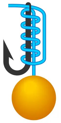
    A knotless knot joining a fishing line (blue) to a fishing hook (grey) and a hair rig (orange)
    Category Hitch
    Related Snell knot
    Typical use Angling

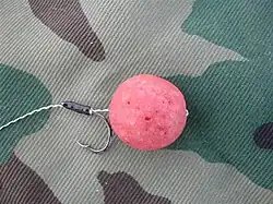
    The knotless knot is a hitch knot used to attach an eyed fishing hook to fishing line while leaving a length of line hanging below the hook.[1] The extra length of line can then be used as the hair of a hair rig.[2]

    Description

    Knotless knot
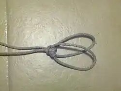
    Knot in use

    The knotless knot is usually tied to a leader, rather than directly to the main line. The far end of the leader may already be baited or looped in preparation for bait, because the knot will be tied using the near end as the working end.

    The working end is passed through the hook eye from back to front (towards the hook point), wrapped tightly around itself and the hook shaft several times (down from the eye towards the bend of the hook), and finally passed once more through the eye back to front.[3]

    References

    External links


    This article is adapted from “Knotless knot” on Wikipedia, written by its contributors, and used under CC BY-SA 4.0. Text on this page is available under the same licence. Source snapshot: Wikipedia via Kiwix, 2026-07-20.

  • Knot thickness

    In knot theory, each link and knot can have an assigned knot thickness. Each realization of a link or knot has a thickness assigned to it. The thickness τ of a link allows us to introduce a scale with respect to which we can then define the ropelength of a link.

    Definition

    There exist several possible definitions of thickness that coincide for smooth enough curves.

    Global radius of curvature

    The thickness is defined using the simpler concept of the local thickness τ(x). The local thickness at a point x on the link is defined as

    τ ( x ) = inf r ( x , y , z ) , {\displaystyle \tau (x)=\inf r(x,y,z),\,} {\displaystyle \tau (x)=\inf r(x,y,z),\,}

    where x, y, and z are points on the link, all distinct, and r(x, y, z) is the radius of the circle that passes through all three points (x, y, z). From this definition we can deduce that the local thickness is at most equal to the local radius of curvature.

    The thickness of a link is defined as

    τ ( L ) = inf τ ( x ) . {\displaystyle \tau (L)=\inf \tau (x).} {\displaystyle \tau (L)=\inf \tau (x).}[1]

    Injectivity radius

    This definition ensures that a normal tube to the link with radius equal to τ(L) will not self intersect, and so we arrive at a “real world” knot made out of a thick string.[2]

    References

    1. “O. Gonzalez, J.H. Maddocks, “Global Curvature, Thickness and the Ideal Shapes of Knots”, Proc. National Academy of Sciences of the USA 96 (1999) 4769–4773″. Archived from the original on 2011-07-06. Retrieved 2009-05-08.
    2. Litherland, R. A.; Simon, J.; Durumeric, O.; Rawdon, E. (1999-02-24). “Thickness of knots”. Topology and Its Applications. 91 (3): 233–244. doi:10.1016/S0166-8641(97)00210-1.


    This article is adapted from “Knot thickness” on Wikipedia, written by its contributors, and used under CC BY-SA 4.0. Text on this page is available under the same licence. Source snapshot: Wikipedia via Kiwix, 2026-07-20.

  • Knot operation

    In knot theory, a knot move or operation is a change or changes which preserve crossing number.[1] Operations are used to investigate whether knots are equivalent, prime or reduced.

    Knot moves or operations include the flype, Habiro move, Markov moves (I. conjugation and II. stabilization), pass move, Perko move, and Reidemeister moves (I. twist move, II. poke move, and III. slide move).[1]

    See also

    References

    1. 1 2 Weisstein, Eric W. “Knot Move”. MathWorld.


    This article is adapted from “Knot operation” on Wikipedia, written by its contributors, and used under CC BY-SA 4.0. Text on this page is available under the same licence. Source snapshot: Wikipedia via Kiwix, 2026-07-20.

  • Knot energy

    In physical knot theory, a knot energy is a functional on the space of all knot conformations. A conformation of a knot is a particular embedding of a circle into three-dimensional space. Depending on the needs of the energy function, the space of conformations is restricted to a sufficiently nicely behaved class. For example, one may consider only polygonal circles or C2 functions. A property of the functional often requires that evolution of the knot under gradient descent does not change knot type.

    Definition

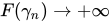
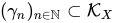
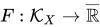
    Let X {\displaystyle X} {\displaystyle X} be a subspace of C ( S 1 , R 3 ) {\displaystyle C(\mathbb {S} ^{1},\mathbb {R} ^{3})} {\displaystyle C(\mathbb {S} ^{1},\mathbb {R} ^{3})} or of C ( S 1 , S 3 ) {\displaystyle C(\mathbb {S} ^{1},\mathbb {S} ^{3})} {\displaystyle C(\mathbb {S} ^{1},\mathbb {S} ^{3})} with a topology (for example C 1 {\displaystyle C^{1}} {\displaystyle C^{1}} or some Sobolev-space with appropriate regularity) and let K X := { γ X : γ  is a topological embedding } {\displaystyle {\mathcal {K}}_{X}:=\{\gamma \in X:\gamma {\text{ is a topological embedding}}\}} {\displaystyle {\mathcal {K}}_{X}:=\{\gamma \in X:\gamma {\text{ is a topological embedding}}\}}. A functional F : K X R ¯ {\displaystyle F:{\mathcal {K}}_{X}\rightarrow {\overline {\mathbb {R} }}} {\displaystyle F:{\mathcal {K}}_{X}\rightarrow {\overline {\mathbb {R} }}} is called self-repulsive with respect topology on X {\displaystyle X} {\displaystyle X} if F ( γ n ) + {\displaystyle F(\gamma _{n})\rightarrow +\infty } {\displaystyle F(\gamma _{n})\rightarrow +\infty } for all sequences ( γ n ) n N K X {\displaystyle (\gamma _{n})_{n\in \mathbb {N} }\subset {\mathcal {K}}_{X}} {\displaystyle (\gamma _{n})_{n\in \mathbb {N} }\subset {\mathcal {K}}_{X}} converging to an immersion with double point with respect to the topology on X {\displaystyle X} {\displaystyle X}.

    A functional F : K X R ¯ {\displaystyle F:{\mathcal {K}}_{X}\rightarrow {\overline {\mathbb {R} }}} {\displaystyle F:{\mathcal {K}}_{X}\rightarrow {\overline {\mathbb {R} }}} is a knot energy if and only if F {\displaystyle F} {\displaystyle F} is a self-repulsive functional and bounded from below.

    Electrical charge

    The most common type of knot energy comes from the intuition of the knot as electrically charged. Coulomb’s law states that two electric charges of the same sign will repel each other as the inverse square of the distance. Thus the knot will evolve under gradient descent according to the electric potential to an ideal configuration that minimizes the electrostatic energy. Naively defined, the integral for the energy will diverge and a regularization trick from physics, subtracting off a term from the energy, is necessary. In addition the knot could change knot type under evolution unless self-intersections are prevented.

    Variations

    An electrostatic energy of polygonal knots was studied by Fukuhara in 1987[1] and shortly after a different, geometric energy was studied by Sakuma.[2][3] In 1988, Jun O’Hara defined a knot energy based on electrostatic energy, Möbius energy.[4] A fundamental property of the O’Hara energy function is that infinite energy barriers exist for passing the knot through itself. With some additional restrictions, O’Hara showed there were only finitely many knot types with energies less than a given bound. Later, Freedman, He, and Wang removed these restrictions.[5]

    Another type of knot energy arises from a more geometric idea. For example, the tangent point energies, first defined by Gonzalez and Maddocks.[6] There, one double-integrate the inverse of the radius of the smallest circle being tangent at one point and passing through another point over the whole curve.[7]

    A similar kind of knot energies is given by the integral Menger curvature. There, one investigates the inverse of the radius the circle passing through three points of the knot and integrates this (three times) over the whole knot.

    References

    1. Fukuhara, Shinji (1988), “Energy of a knot”, A fête of topology, Academic Press, Boston, MA, pp. 443–451, MR 0928412.
    2. Sakuma, M. (1987), “Problem no. 8”, in Kojima, S.; Negami, S. (eds.), The collection of problems on “Low dimensional topology and related matters” (in Japanese), p. 7. As cited by Langevin & O’Hara (2005).
    3. Langevin, R.; O’Hara, J. (2005), “Conformally invariant energies of knots”, Journal of the Institute of Mathematics of Jussieu, 4 (2): 219–280, arXiv:math.GT/0409396, doi:10.1017/S1474748005000058, MR 2135138.
    4. O’Hara, Jun (1991), “Energy of a knot”, Topology, 30 (2): 241–247, doi:10.1016/0040-9383(91)90010-2, MR 1098918.
    5. Freedman, Michael H.; He, Zheng-Xu; Wang, Zhenghan (1994), “Möbius energy of knots and unknots”, Annals of Mathematics, Second Series, 139 (1): 1–50, doi:10.2307/2946626, MR 1259363.
    6. Gonzalez, Oscar; Maddocks, John H. (1999). “Global Curvature, Thickness, and the Ideal Shapes of Knots”. Proceedings of the National Academy of Sciences of the United States of America. 96 (9): 4769–4773. ISSN 0027-8424.
    7. Blatt, Simon; Reiter, Philipp (2015-04-01). “Regularity theory for tangent-point energies: The non-degenerate sub-critical case”. Advances in Calculus of Variations. 8 (2): 93–116. arXiv:1208.3605. doi:10.1515/acv-2013-0020. ISSN 1864-8266.

    This article is adapted from “Knot energy” on Wikipedia, written by its contributors, and used under CC BY-SA 4.0. Text on this page is available under the same licence. Source snapshot: Wikipedia via Kiwix, 2026-07-20.

  • Kinoshita–Terasaka knot

    Kinoshita–Terasaka knot
    Crossing no. 11
    Genus 2
    Hyperbolic volume 11.2191
    Thistlethwaite 11n42
    Other
    prime, prime, slice
    Kinoshita–Terasaka knot
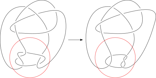
    The prime Kinoshita–Terasaka knot (11n42) (left) and the prime Conway knot (11n34) (right) showing how they are related by mutation

    In knot theory, the Kinoshita–Terasaka knot is a particular prime knot with 11 crossings.[1] It is named after Japanese mathematicians Shinichi Kinoshita and Hidetaka Terasaka, who wrote about it in 1957.[2] The Kinoshita–Terasaka knot has a variety of interesting mathematical properties.[3] It is related by mutation to the Conway knot,[4] with which it shares a Jones polynomial. It has the same Alexander polynomial as the unknot.[5]

    References

    1. Weisstein, Eric W. “Conway’s Knot”. mathworld.wolfram.com. Retrieved 2020-05-19.
    2. Kinoshita, S.; Terasaka, H. (1957). “On Unions of Knots”. Osaka Math J. 9: 131–153.
    3. Tillmann, Stephan (June 2000). “On the Kinoshita-Terasaka knot and generalised Conway mutation” (PDF). Journal of Knot Theory and Its Ramifications. 09 (4): 557–575. doi:10.1142/S0218216500000311. ISSN 0218-2165.
    4. Chmutov, S.V. (2007). “Mutant Knots” (PDF). people.math.osu.edu. Archived from the original (PDF) on 2020-06-12.
    5. Boi, Luciano (2 November 2005). Geometries of Nature, Living Systems and Human Cognition: New Interactions of Mathematics with Natural Sciences and Humanities. ISBN 9789814479455.

    External links


    This article is adapted from “Kinoshita–Terasaka knot” on Wikipedia, written by its contributors, and used under CC BY-SA 4.0. Text on this page is available under the same licence. Source snapshot: Wikipedia via Kiwix, 2026-07-20.

  • Khovanov homology

    In mathematics, Khovanov homology is an oriented link invariant that arises as the cohomology of a cochain complex. It may be regarded as a categorification of the Jones polynomial.

    It was developed in the late 1990s by Mikhail Khovanov.

    Overview

    To any link diagram D {\displaystyle D} {\displaystyle D} representing a link L {\displaystyle L} {\displaystyle L}, we assign the Khovanov bracket [ D ] {\displaystyle \left[D\right]} {\displaystyle \left[D\right]}, a cochain complex of graded vector spaces. This is the analogue of the Kauffman bracket in the construction of the Jones polynomial. Next, we normalise [ D ] {\displaystyle \left[D\right]} {\displaystyle \left[D\right]} by a series of degree shifts (in the graded vector spaces) and height shifts (in the cochain complex) to obtain a new cochain complex C ( D ) {\displaystyle C(D)} {\displaystyle C(D)}. The cohomology of this cochain complex turns out to be an invariant of L {\displaystyle L} {\displaystyle L}, and its graded Euler characteristic is the Jones polynomial of L {\displaystyle L} {\displaystyle L}.

    Definition

    This definition follows the formalism given in Dror Bar-Natan’s 2002 paper.

    Let l {\displaystyle l} {\displaystyle l} denote the degree shift operation on graded vector spacesthat is, the homogeneous component in dimension m {\displaystyle m} {\displaystyle m} is shifted up to dimension m + l {\displaystyle m+l} {\displaystyle m+l}.

    Similarly, let [ s ] {\displaystyle [s]} {\displaystyle [s]} denote the height shift operation on cochain complexes—that is, the r {\displaystyle r} {\displaystyle r}th vector space or module in the complex is shifted along to the ( r + s ) {\displaystyle (r+s)} {\displaystyle (r+s)}th place, with all the differential maps being shifted accordingly.

    Let V {\displaystyle V} {\displaystyle V} be a graded vector space with one generator q {\displaystyle q} {\displaystyle q} of degree 1, and one generator q 1 {\displaystyle q^{-1}} {\displaystyle q^{-1}} of degree  1 {\displaystyle -1} {\displaystyle -1}.

    Now take an arbitrary diagram D {\displaystyle D} {\displaystyle D} representing a link L {\displaystyle L} {\displaystyle L}. The axioms for the Khovanov bracket are as follows:

    1. [ ] = ( 0 Z 0 ) {\displaystyle [\emptyset ]=(0\to \mathbb {Z} \to 0)} {\displaystyle [\emptyset ]=(0\to \mathbb {Z} \to 0)}, where {\displaystyle \emptyset } {\displaystyle \emptyset } denotes the empty link.
    2. [ D ] = V [ D ] {\displaystyle [{\text{O }}D]=V\otimes [D]} {\displaystyle [{\text{O }}D]=V\otimes [D]}, where O denotes an unlinked trivial component.
    3. [ D ] = F ( 0 [ D 0 ] [ D 1 ] { 1 } 0 ) {\displaystyle [D]=\mathbf {F} (0\to [D_{0}]\to [D_{1}]\{1\}\to 0)} {\displaystyle [D]=\mathbf {F} (0\to [D_{0}]\to [D_{1}]\{1\}\to 0)}

    In the third of these, F {\displaystyle \mathbf {F} } {\displaystyle \mathbf {F} } denotes the `flattening’ operation, where a single complex is formed from a double complex by taking direct sums along the diagonals. Also, D 0 {\displaystyle D_{0}} {\displaystyle D_{0}} denotes the `0-smoothing’ of a chosen crossing in D {\displaystyle D} {\displaystyle D}, and D 1 {\displaystyle D_{1}} {\displaystyle D_{1}} denotes the `1-smoothing’, analogously to the skein relation for the Kauffman bracket.

    Next, we construct the `normalised’ complex C ( D ) = [ D ] [ n ] { n + 2 n } {\displaystyle \mathbf {C} (D)=[D][-n_{-}]\{n_{+}-2n_{-}\}} {\displaystyle \mathbf {C} (D)=[D][-n_{-}]\{n_{+}-2n_{-}\}}, where n {\displaystyle n_{-}} {\displaystyle n_{-}} denotes the number of left-handed crossings in the chosen diagram for D {\displaystyle D} {\displaystyle D}, and n + {\displaystyle n_{+}} {\displaystyle n_{+}} the number of right-handed crossings.

    The Khovanov homology of L {\displaystyle L} {\displaystyle L} is then defined as the cohomology H ( L ) {\displaystyle \mathbf {H} (L)} {\displaystyle \mathbf {H} (L)} of this complex C ( D ) {\displaystyle \mathbf {C} (D)} {\displaystyle \mathbf {C} (D)}. It turns out that the Khovanov homology is indeed an invariant of L {\displaystyle L} {\displaystyle L}, and does not depend on the choice of diagram. The graded Euler characteristic of H ( L ) {\displaystyle \mathbf {H} (L)} {\displaystyle \mathbf {H} (L)} turns out to be the Jones polynomial of L {\displaystyle L} {\displaystyle L}. However, H ( L ) {\displaystyle \mathbf {H} (L)} {\displaystyle \mathbf {H} (L)} has been shown to contain more information about L {\displaystyle L} {\displaystyle L} than the Jones polynomial, but the exact details are not yet fully understood.

    In 2006 Dror Bar-Natan developed a computer program to calculate the Khovanov homology (or category) for any knot.[1]

    Related theories

    One of the most interesting aspects of Khovanov’s homology is that its exact sequences are formally similar to those arising in the Floer homology of 3-manifolds. Moreover, it has been used to produce another proof of a result first demonstrated using gauge theory and its cousins: Jacob Rasmussen’s new proof of a theorem of Peter Kronheimer and Tomasz Mrowka, formerly known as the Milnor conjecture (see below). There is a spectral sequence relating Khovanov homology with the knot Floer homology of Peter Ozsváth and Zoltán Szabó (Dowlin 2018).[2] This spectral sequence settled an earlier conjecture on the relationship between the two theories (Dunfield et al. 2005). Another spectral sequence (Ozsváth-Szabó 2005) relates a variant of Khovanov homology with the Heegaard Floer homology of the branched double cover along a knot. A third (Bloom 2009) converges to a variant of the monopole Floer homology of the branched double cover. In 2010 Kronheimer and Mrowka [3] exhibited a spectral sequence abutting to their instanton knot Floer homology group and used this to show that Khovanov Homology (like the instanton knot Floer homology) detects the unknot.

    Khovanov homology is related to the representation theory of the Lie algebra s l 2 {\displaystyle {\mathfrak {sl}}_{2}} {\displaystyle {\mathfrak {sl}}_{2}}. Mikhail Khovanov and Lev Rozansky have since defined homology theories associated to s l n {\displaystyle {\mathfrak {sl}}_{n}} {\displaystyle {\mathfrak {sl}}_{n}} for all n {\displaystyle n} {\displaystyle n}. In 2003, Catharina Stroppel extended Khovanov homology to an invariant of tangles (a categorified version of Reshetikhin-Turaev invariants) which also generalizes to s l n {\displaystyle {\mathfrak {sl}}_{n}} {\displaystyle {\mathfrak {sl}}_{n}} for all n {\displaystyle n} {\displaystyle n}.
    Paul Seidel and Ivan Smith have constructed a singly graded knot homology theory using Lagrangian intersection Floer homology, which they conjecture to be isomorphic to a singly graded version of Khovanov homology. Ciprian Manolescu has since simplified their construction and shown how to recover the Jones polynomial from the cochain complex underlying his version of the SeidelSmith invariant.

    The relation to link (knot) polynomials

    At International Congress of Mathematicians in 2006 Mikhail Khovanov provided the following explanation for the relation to knot polynomials from the view point of Khovanov homology. The skein relation for three links L 1 , L 2 {\displaystyle L_{1},L_{2}} {\displaystyle L_{1},L_{2}} and L 3 {\displaystyle L_{3}} {\displaystyle L_{3}} is described as

    λ P ( L 1 ) λ 1 P ( L 2 ) = ( q q 1 ) P ( L 3 ) . {\displaystyle \lambda P(L_{1})-\lambda ^{-1}P(L_{2})=(q-q^{-1})P(L_{3}).} {\displaystyle \lambda P(L_{1})-\lambda ^{-1}P(L_{2})=(q-q^{-1})P(L_{3}).}

    Substituting λ = q n , n 0 {\displaystyle \lambda =q^{n},n\leq 0} {\displaystyle \lambda =q^{n},n\leq 0} leads to a link polynomial invariant P n ( L ) Z [ q , q 1 ] {\displaystyle P_{n}(L)\in \mathbb {Z} [q,q^{-1}]} {\displaystyle P_{n}(L)\in \mathbb {Z} [q,q^{-1}]}, normalized so that

    P n ( u n k n o t ) = q n 1 + q n 3 + + q 1 n n > 0 P 0 ( u n k n o t ) = 1 {\displaystyle {\begin{aligned}P_{n}(unknot)&=q^{n-1}+q^{n-3}+\cdots +q^{1-n}&&n>0\\P_{0}(unknot)&=1\end{aligned}}} {\displaystyle {\begin{aligned}P_{n}(unknot)&=q^{n-1}+q^{n-3}+\cdots +q^{1-n}&&n>0\\P_{0}(unknot)&=1\end{aligned}}}

    For n > 1 {\displaystyle n>1} {\displaystyle n>1} the polynomial P n ( L ) {\displaystyle P_{n}(L)} {\displaystyle P_{n}(L)} can be interpreted via the representation theory of quantum group U q ( s l ( n ) ) {\displaystyle U_{q}(sl(n))} {\displaystyle U_{q}(sl(n))} and P 0 ( L ) {\displaystyle P_{0}(L)} {\displaystyle P_{0}(L)} via that of the quantum Lie superalgebra U q ( g l ( 1 | 1 ) ) {\displaystyle U_{q}(gl(1|1))} {\displaystyle U_{q}(gl(1|1))}.

    • The Alexander polynomial P 0 ( L ) {\displaystyle P_{0}(L)} {\displaystyle P_{0}(L)} is the Euler characteristic of a bigraded knot homology theory.
    • P 1 ( L ) = 1 {\displaystyle P_{1}(L)=1} {\displaystyle P_{1}(L)=1} is trivial.
    • The Jones polynomial P 2 ( L ) {\displaystyle P_{2}(L)} {\displaystyle P_{2}(L)} is the Euler characteristic of a bigraded link homology theory.
    • The entire HOMFLY-PT polynomial is the Euler characteristic of a triply graded link homology theory.

    Applications

    The first application of Khovanov homology was provided by Jacob Rasmussen, who defined the s-invariant using Khovanov homology. This integer valued invariant of a knot gives a bound on the slice genus, and is sufficient to prove the Milnor conjecture.

    In 2010, Kronheimer and Mrowka proved that the Khovanov homology detects the unknot. The categorified theory has more information than the non-categorified theory. Although the Khovanov homology detects the unknot, it is not yet known if the Jones polynomial does.

    Notes

    1. New Scientist, 18 October 2008
    2. Dowlin, Nathan (2018-11-19). “A spectral sequence from Khovanov homology to knot Floer homology”. arXiv:1811.07848 [math.GT].
    3. Kronheimer, Peter B.; Mrowka, Tomasz (2011). “Khovanov homology is an unknot-detector”. Publications Mathématiques de l’IHÉS. 113: 97–208. arXiv:1005.4346. doi:10.1007/s10240-010-0030-y. S2CID 119586228.

    References

    External links


    This article is adapted from “Khovanov homology” on Wikipedia, written by its contributors, and used under CC BY-SA 4.0. Text on this page is available under the same licence. Source snapshot: Wikipedia via Kiwix, 2026-07-20.

  • Karash double loop

    Karash double loop
    Karash double loop
    Category Loop
    Efficiency 49-72% (12.5 mm static)[1]
    Typical use climbing, rope rescue

    Karash double loop is a common name for a knot forming two loops. This knot has been a known variant of the Bowline on a bight per the International Guild of Knot Tyers, referred to as bowline twist or twisted collar bowline on a bight.[2] The knot is also referred to as nœud de fusion in French references and sometimes called Fusion knot in English.

    The name Karash double loop was introduced by Mike Karash, who re-invented the knot to create makeshift harnesses for rescue operations and popularized it among rescue workers.[3][4]

    Applications

    The knot is used for vertical caving using the single rope technique,[5] particularly by French cavers. It is advertised by the French Federation of Speleology as a safe alternative to the bowline on a bight. Compared to the traditional double loop variant of the figure of eight, its loops remain open under load allowing to clip and unclip carabiners in the loops more easily.

    The knot is also popular to create a makeshift harness in rescue operations. The two loops are used as leg loops to sit in. The knot can be further improved by adding two bowlines around a person’s body to create a three-point harness.[6][7]

    Technique

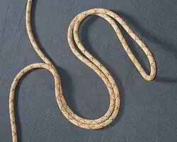
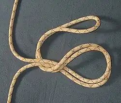
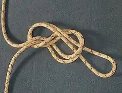
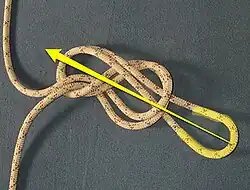
    The traditional method of tying this knot starts with a reverse loop (like the Eskimo bowline) then wraps around the standing end (AKA the “tree”), you then finish the knot the same way as the BOAB – Bowline on a bight.

    An alternative way as advertised by the French Federation of Speleology and Mike Karash is starting with a figure of eight on a bight, then pulls two strands of the rope back through the bight.

    • Start with a bight of rope
      Start with a bight of rope
    • Tie a figure of eight on the bight
      Tie a figure of eight on the bight
    • Karash double loop
    • Pull the loop of the figure of eight over the whole knot
      Pull the loop of the figure of eight over the whole knot
    • Karash double loop
    • Karash double loop
    • Take the two strands of rope together
      Take the two strands of rope together
    • Pull back the two strands of rope closest to the loop inside the knot
      Pull back the two strands of rope closest to the loop inside the knot
    • These two form the final two loops of the knot
      These two form the final two loops of the knot
    • Tighten and dress the knot
      Tighten and dress the knot

    References

    External links


    This article is adapted from “Karash double loop” on Wikipedia, written by its contributors, and used under CC BY-SA 4.0. Text on this page is available under the same licence. Source snapshot: Wikipedia via Kiwix, 2026-07-20.

  • Jury mast knot

    Jury mast knot
    Jury mast knot

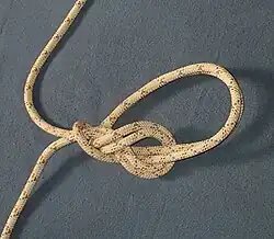
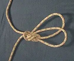
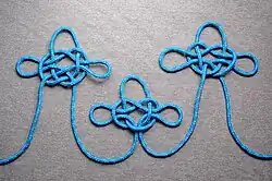
    Three variations of the Jury mast knot
    Names Jury mast knot, Masthead knot, Pitcher Knot, Jury masthead
    Category Loop
    Related Tom fool’s knot, Handcuff knot, Bottle sling
    Typical use Jury rigging a mast, carrying pitchers
    ABoK #1167, #1168, #1169, #2563

    The jury mast knot (or masthead knot) is traditionally presented as to be used for jury rigging a temporary mast on a sailboat or ship after the original one has been lost; some authors claim a use for derrick poles—but there is no good evidence for actual use. The knot is placed at the top of a new mast with the mast projecting through the center of the knot. The loops of the knot are then used as anchor points for makeshift stays and shrouds. Usually small blocks of wood are affixed to, or a groove cut in, the new mast to prevent the knot from sliding downwards.[1]

    Due to a lack of hard historical evidence there is uncertainty whether this supposed rigging knot was ever commonly used for rigging jury masts.[2]

    Variations

    There are three closely related variations of this knot. They differ based on the type of crossing, overhand or underhand, of the three initial loops and then whether the edges of each loop is positioned over or under the previous one. Although these knots are tied in the bight, for the purposes of description the left side will be considered the standing part. If all the crossings and overlays are reversed, or the right side is taken as the standing part, a mirror image of the knot will result.

    #1167

    This variation might grip the mast best (per Ashley) in the absence of other means to prevent the knot from sliding downwards. The pattern of this variation, from the left, is: under-under/over-over.

    Jury mast knot
    Jury mast knot

    #1168

    This variation is the simplest of the three in structure (though not in tying) and lends itself to being reinforced by tying a reef knot with the two free ends. The pattern of this variation, from the left, is: under-over-under/over-over.

    Jury mast knot
    Jury mast knot

    #1169

    The pattern of this variation, from the left, is: under-under-under/under-under.

    Jury mast knot
    Jury mast knot

    References

    1. Clifford W. Ashley, The Ashley Book of Knots (New York: Doubleday, 1944), 212.
    2. Charles Hamel, “Investigations on the Jury Mast Knot” (URLs retrieved 2007-02-22)

    External links


    This article is adapted from “Jury mast knot” on Wikipedia, written by its contributors, and used under CC BY-SA 4.0. Text on this page is available under the same licence. Source snapshot: Wikipedia via Kiwix, 2026-07-20.
  • Infantry Shoulder Cord

    Infantry Shoulder Cord
    Infantry Shoulder Cord
    Type Military insignia
    Awarded for Completion of One Station Unit Training or Advanced Individual Training (enlisted) or completion of U.S. Army Infantry School’s Infantry Officer Basic Course (officers)
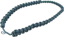
    Description The shoulder cord is infantry blue. It is formed by a series of interlocking square knots around a
    center cord.
    Country Infantry Shoulder Cord United States
    Presented by Secretary of the Army
    Eligibility U.S. Army Infantry personnel
    Status Currently awarded
    Established 1952 (1952)

    The Infantryman Shoulder Cord is a United States military decoration worn over the right shoulder of all infantry-qualified U.S. Army soldiers. It is a fourragere in light blue, specifically PMS 5415 (dubbed “Infantry Blue” by the U.S. Army), worn under the right shoulder and under the right epaulette of a U.S. Army infantry soldier’s Class A dress blue uniform jacket[1] or Class B shirt.[2] The cord is composed of a series of alternating left and right half knots that are tied around a leader cord to form a “Solomon bar”.

    History

    The modern Infantry blue cord is a simplified version of the breast and right shoulder cord worn in 1902 as part of the newly introduced full dress uniform of that date. This ceremonial item was in army, corps or departmental color (light-blue for infantry).[3]
    During the Korean War General J. Lawton Collins, Chief of Staff for the Army, asked a group of advisers what could be done to enhance the morale of the fighting Infantryman. It was decided that they would receive special insignia, so that everyone would know that the soldier was an infantryman who would be fighting on the front lines.

    A light-blue cord was created to be worn on the right shoulder of both infantry trained officers and enlisted men. Also, light-blue plastic disks were issued to be placed behind the metal “crossed rifles” Infantry branch of service insignia U.S. collar discs on Class A and Class B uniforms as well as on the U.S. coat of arms disc on the front of the service cap. The new enhancements were first worn by the 3rd U.S. Infantry Regiment (“The Old Guard”). The light-blue cord and disks became standard for all U.S. infantry soldiers in 1952.

    Qualification

    The infantry blue cord is presented to all infantry-qualified soldiers in the U.S. Army at the end of their Advanced Individual Training. Commissioned officers earn their blue cord after graduating from the U.S. Army Infantry School’s Infantry Officer Basic Course (IBOLC). Enlisted soldiers earn their infantry blue cords after successfully completing all Infantry Training Brigade requirements required for achieving the infantry MOS by graduating from 22 weeks of Infantry One Station Unit Training (OSUT), or twelve weeks of Infantry Advanced Individual Training (AIT) for those who go through “Basic” and AIT via Split Training Option (Split-Op) which is conducted at the United States Army Infantry School at Fort Benning, Georgia.

    The infantry blue cord is authorized to be worn only by infantry-qualified U.S. Army soldiers currently assigned to an infantry unit in the active U.S. Army, U.S. Army Reserve, or Army National Guard. Only those with an infantry military occupational specialty such as 11A (infantry officers), 11B, or 11C. Other 11 series MOS holders (as both their primary and duty MOS) who may wear the cord are infantry soldiers assigned to an infantry slot that is not in an infantry unit (such as with infantry assigned to a cavalry unit) if authorized, or instructors, drill sergeants, or recruiters. Individuals holding the 11X designator do not wear the cord as this is an “unassigned” position designated for recruits who are contracted into the CMF (Career Management Field) 11 – Infantry.

    Qualified infantry soldiers who are not assigned to an infantry unit, to include those who are an 11-series MOS holder transitioning to 18-series MOS, for example, (CMF 18 is the designation for the Army Special Forces MOS) may not wear the infantry blue cord or disks. Those soldiers who are assigned to an infantry unit may wear the infantry blue cord and disks until their transition to a non-Infantry unit is complete.

    Presentation

    Infantry Shoulder Cord
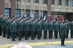
    Newly qualified infantrymen receive their infantry blue cords at a “Turning Blue” ceremony in 2009, following 16 weeks of One Station Unit Training (OSUT), the day before graduation in front of their barracks at Fort Benning.

    Today, enlisted graduates of infantry “One Station Unit Training” or “Split Training Option” receive their blue cord at the “Turning Blue” ceremony held the day before their graduation from Infantry advanced individual training (AIT). This ceremony typically follows a week-long field training exercise (FTX) including at least a 5-mile ruck march to the field, multiple force on force and team exercises that precede at least a 12-mile ruck march back to garrison. All other recruits first attend a 9-week basic combat training (BCT) course before moving on to their AIT in which they will have a similar ceremony. However, only those who have graduated the infantry school and maintain postings in infantry units OR certain branch immaterial units (i.e.: Drill Sergeant, Branch Detailed Recruiters, etc…) are authorized to wear the blue cord.

    Graduates of the Infantry Basic Officer Leaders Course (formerly IOBC) must complete their two-week-long final FTX with a 16-mile tactical road march and a mock company attack. Prior to graduation and out-processing, students have their “Blue Cord” ceremony at Freedom Hall where their blue cords are pinned on them by their platoon trainer captain and NCOs. The staff sergeant or sergeant first class who pins on the blue cord then renders a salute recognizing the lieutenant’s entry into the ranks of the infantry.

    See also

    References

    1. “First Gender-Integrated Infantry One Station Unit Training Company Graduates”. www.army.mil. 2017.
    2. Ledger-Enquirer, Chuck Williams, Columbus (19 May 2017). “18 Women Graduate From Army’s Enlisted Infantry Training”. Task & Purpose. Archived from the original on 7 December 2018. Retrieved 7 December 2018.{{cite web}}: CS1 maint: multiple names: authors list (link)
    3. Section 68, “Regulations and Notes for the Uniform of the Army of the United States 1902”

    Further reading

    • AR 670-1, Wear and Appearance of Army Uniforms and Insignia (pp. 28–30. “Distinctive items authorized for infantry personnel”).

    External links


    This article is adapted from “Infantry Shoulder Cord” on Wikipedia, written by its contributors, and used under CC BY-SA 4.0. Text on this page is available under the same licence. Source snapshot: Wikipedia via Kiwix, 2026-07-20.