This page explains commonly used terms related to knots.
B
Bend
A bend is a knot used to join two lengths of rope.
Bight
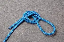
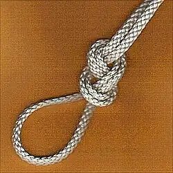
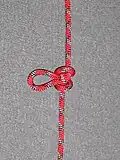
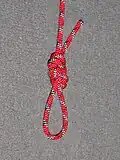
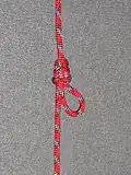
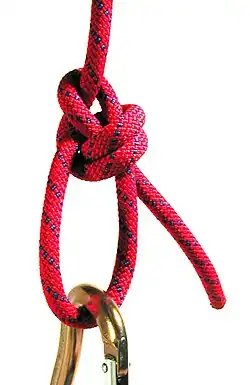
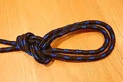
When an overhand knot is tied with a bight instead of an end of the rope, the result is an overhand loop
A bight is a slack part in the middle of a rope, usually a curve or loop.[1][2] Knots that can be tied without access to either end of the rope are called knots in the bight. To tie a knot with a bight is to double up the rope into a bight and then tie the knot using the double rope.
Binding knot
Binding knots are knots that either constrict a single object or hold two objects snugly together. Whippings, seizings and lashings serve a similar purpose to binding knots, but contain too many wraps to be properly called a knot.[1] In binding knots, the ends of rope are either joined together or tucked under the turns of the knot.
Bitter end
Another term for the working end.[3] In its original meaning, and still today in strict nautical meaning, the bitter end was the opposite end of a rope or cable, from the working end, and not the same. The name comes from the “bitts” or “cable bitts”, which were fixtures comprising a pair of strongly fixed posts used on wooden sailing ships to attach the inboard end of the anchor cable.[4] The outboard end of a rope or cable, on the contrary, is the “working end”. The phrase “to reach the bitter end” is a metaphor for reaching the end of the anchor cable; paying it out until there is no more left.[5]
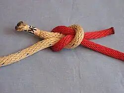
A knot that has capsized or spilled has deformed into a different structure. Although capsizing is sometimes the result of incorrect tying or misuse, it can also be done purposefully in certain cases to strengthen the knot (see the carrick bend[6]) or to untie a seized knot which would otherwise be difficult to release (see reef knot).
Chirality
Chirality is the ‘handedness’ of a knot. Topologically speaking, a knot and its mirror image may or may not have knot equivalence.[7]
D
Decorative knot
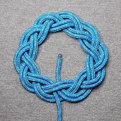
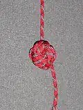
Although primarily tied for decorative purposes, the Turk’s head knot can serve as a hand grip when tied around a cylindrical object.[8]
A decorative knot is any aesthetically pleasing knot. Although it is not necessarily the case, most decorative knots also have practical applications or were derived from other well-known knots.[8] Decorative knotting is one of the oldest and most widely distributed types of folk art.[8]
Dressing
Knot dressing is the process of arranging a knot in such a way as to improve its performance. Crossing or uncrossing the rope in a specific way, depending on the knot, can increase the knot’s strength as well as reduce its jamming potential.[9]
E
Elbow
An elbow refers to any two nearby crossings of a rope. An elbow is created when an additional twist is made in a loop.[10]
Eye
The eye is in fact what is often (in error) referred to as a loop.
The eye functions in the same way as an eye bolt or an eye splice. The eye provides a means to form connections. The eye of a knot (or a splice) is fixed and does not slip. If it slipped, it would not function as an eye – it would act like a noose.
F
Flake
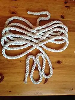
A flake refers to any number of turns in a coiled rope. Likewise, to flake a rope means to coil it.[1]
“Flaking” or “Faking” also means to lay a rope on a surface ready to use or to run out quickly without tangles.[11]
Figure-8 flake
Fraps
Fraps or “frapping turns” are a set of loops coiled perpendicularly around the wraps of a lashing as a means of tightening.[12]
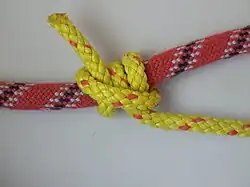
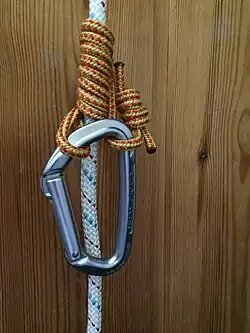
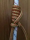
The rolling hitch is a common type of friction hitch.
Friction hitch
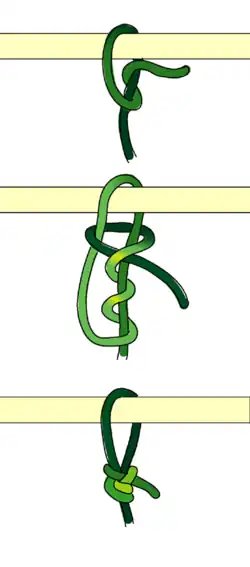
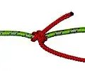
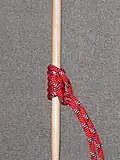
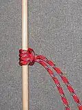
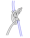
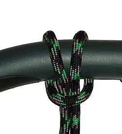
A friction hitch is a knot that attaches one rope to another in a way that allows the knot’s position to easily be adjusted. Sometimes friction hitches are called slide-and-grip knots.[13] They are often used in climbing applications.
H
Hitch
A hitch is a knot that attaches a rope to some object, often a ring, rail, spar, post, or perhaps another rope, as in the case of the rolling hitch.[14]
J
Jamming
A jamming knot is any knot that becomes very difficult to untie after use.[15] Knots that are resistant to jamming are called non-jamming knots. Jamming knots include #1230, #1727, and #1994 in The Ashley Book of Knots.
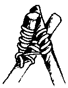
A lashing is an arrangement of rope used to secure two or more items together in a rigid manner. Common uses include the joining of scaffolding poles and the securing of sailing masts.[16][17] The square lashing, diagonal lashing, and shear lashing are well-known lashings used to bind poles perpendicularly, diagonally, and in parallel, respectively.[18]
Loop
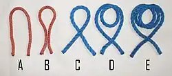
A: open loop, B: closed loop, C: turn, D: round turn, and E: two round turns
In reference to knots, loop may refer to:
One of the fundamental structures used to tie knots. Specifically, it is a U-form narrower than a bight.[19]
A type of knot used to create a closed circle in a line.
A loop is one of the fundamental structures used to tie knots. It is a full circle formed by passing the working end of a rope over itself. When the legs of a closed loop are crossed to form a loop, the rope has taken a turn.[1]
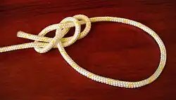
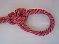
A loop knot is a type of knot that creates a fixed loop on the rope, where “fixed” means that pulling on the rope does not cause the loop to slide or shrink. In contrast to a hitch, the loop formed by a loop knot maintains its structure regardless of whether or not the loop is around an object.[1]
A loop can be formed by tying “in the bight” or otherwise. An example is the figure-eight loop knot, which can be tied in the bight, by tying a figure-eight knot using a bight instead of the end of the rope. However, tying the knot this way does not allow putting the loop around a fixed object like a tree; to do that, the knot must be tied in a two-stage process by first tying a figure-eight knot, running the end of the rope around the fixed object, and then threading the rope back through and around the figure-8 knot to create the final figure-8 loop knot.
N
Noose
A noose can refer to any sliding loop in which the loop tightens when pulled.[6]
O
Open loop
An open loop is a curve in a rope that resembles a semicircle in which the legs are not touching or crossed. The legs of an open loop are brought together narrower than they are in a bight.[1]
S
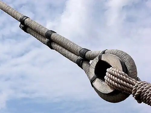
The eye of a forestay is secured by three round seizings
Seizing
A seizing is a knot that binds two pieces of rope together side by side, normally in order to create a loop. The structure of seizings is similar to that of lashings.[20]
Setting
Setting a knot is the process of tightening it. Improper setting can cause certain knots to underperform.[9]
Slipped knot
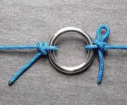
The slipped form of the buntline hitch (on the right) can easily be untied by pulling the hanging end and withdrawing the loop.
A slipped knot is any knot that unties when an end is pulled. Thus, tying the slipped form of a knot makes it easier to untie, especially when the knot is prone to jamming.[1] A slip knot is just one variety of slipped knot.
Small-stuff
Small-stuff is a nautical and knot-tying term for thin string or twine, as opposed to the thick, heavy ropes that are more often used in sailing. It is commonly used in a whipping to bind the ends of ropes to prevent fraying.
Historically, the term referred to cordage less than one inch in circumference.[21] Much of the small-stuff on board ships, especially that used for decorative or fancy ropework, was made by the sailors themselves reusing materials unlaid from old and leftover pieces of larger rope and cable.[22]
Spilling
Splice
Splicing is a method of joining two ropes done by untwisting and then re-weaving the rope’s strands.[23]
Standing end
The standing end (or standing part) of a rope is the part that is not active in knot tying.[1] The opposite end is the working end.[6]
Stopper knot
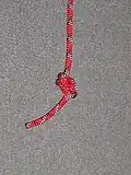
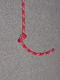
A stopper knot is the type of knot tied to prevent a rope from slipping through a grommet.[24] The overhand knot is the simplest single-strand stopper knot.[1]
T
Turn
A turn is one round of rope on a pin or cleat, or one round of a coil.
W
Whipping
A whipping is a binding knot tied around the end of a rope to prevent the rope from unraveling.[20]
Working end
The working end (or working part) of a rope is the part active in knot tying.[1] The opposite end is the standing end.[6]
12345678910Ashley, Clifford W. (1993) [reprinted, first printing 1944]. The Ashley Book of Knots. New York: Doubleday. pp.11–20, 219, 597–599. ISBN0-385-04025-3. “Any slack part of a rope between the two ends, particularly when curved or looped.”
↑“Rope and Knot Terminology”. Upper Ojai Search and Rescue Team. Ventura Country Sheriff’s Department. Retrieved 19 July 2011.
↑Hasluck, Paul N., ed. (October 15, 2009). Knotting And Splicing Ropes And Cordage. Kessinger Publishing, LLC. p.130. ISBN978-1-120-30885-6.
↑Biddlecombe, George (1990). The Art of Rigging (1ed.). Mineola, New York. p.19. ISBN0-486-26343-6.{{cite book}}: CS1 maint: location missing publisher (link)
↑Macfarlan, Allan and Paulette (September 1, 1983). Knotcraft: The Practical and Entertaining Art of Tying Knots. Dover Publications. ISBN0-486-24515-2.
↑Clifford W. Ashley, The Ashley Book of Knots. Image 31, 32.
12Merry, Barbara; Martin Dugard (February 16, 2000). The Splicing Handbook: Techniques for Modern and Traditional Ropes (2ed.). International Marine/Ragged Mountain Press. p.113. ISBN978-0-07-135438-7.
↑Clifford W. Ashley, The Ashley Book of Knots (New York: Doubleday, 1944), 603.
↑Wing, Charlie (May 2007). How Boat Things Work: An Illustrated Guide. McGraw-Hill. p.97. ISBN978-0-07-149344-4.
This article is adapted from “List of knot terminology” on Wikipedia, written by its contributors, and used under CC BY-SA 4.0. Text on this page is available under the same licence. Source snapshot: Wikipedia via Kiwix, 2026-07-20.
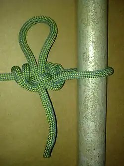
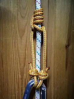
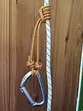
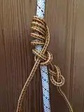
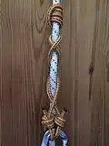
A friction hitch is a kind of knot used to attach one rope to another in a way that is easily adjusted. These knots are commonly used in climbing as part of single-rope technique, doubled-rope technique and as “ratchets” to capture progress on a moving rope, most typically in a mechanical advantage system such as a Z-drag. These hitches are a simple and cheap alternative to mechanical ascenders.
A friction hitch tied around a thicker rope that can slide while unloaded, but locks when loaded. Commonly used to back up belays. Similar to the Prusik only in function. French Prusik is equivalent to bi-directional Machard.
A friction hitch commonly used by arborists and tree climbers as an ascending knot. Blake’s hitch is known by some climbers as a Swicero (Suicero) knot or Verones knot.
A slip and grip knot that gives good grip and has a wide range of use. Functions well on a wide range of rope materials, including slippery types like polyamide (nylon) and high-modulus polyethylene (Dynema™). Attaching cord can be of same or smaller diameter. Grip in one direction.
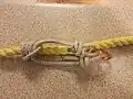
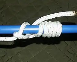
A secure, jam-proof hitch used to tie one rope to another, or a rope to a pole, boom, spar, etc., when the pull is lengthwise along the object. It is also known as Michoacan/Martin among friction knots used in climbing.
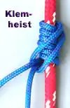
A friction hitch tied around a thicker rope that can slide while unloaded, but locks when loaded. Similar to the Prusik. Klemheist knot is a full equivalent to uni-directional Machard.
Knut hitch
A friction hitch used for climbing a rope, not to be confused with the Knute hitch.[1]
Machard Tresse
A mono-directional variant of the common Machard. Tresse, French for braided, indicates a final crossing turn, which increases the hitch’s hold and ease of release.
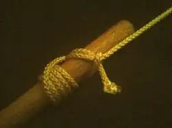
A friction hitch tied around a thicker rope that can slide while unloaded, but locks when loaded.[2][3] Similar to the Prusik. Michoacan/Martin is a full equivalent to Gripping sailor’s hitch
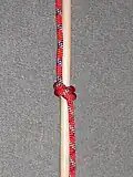
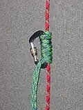
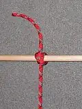
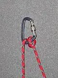
A friction hitch or knot used to put a loop of cord around a rope, applied in climbing, canyoneering, mountaineering, caving, rope rescue, and by arborists.
A friction hitch tied around a thicker rope that can slide while unloaded, but locks when loaded. Similar to the Prusik
Todd-Kramer hitch
A friction hitch tied around a thicker rope that can slide while unloaded, but locks when loaded. Similar to the Prusik
Valdotain Tresse
Friction knot used to be fixed on a tautline (a taut-rope), also known as a “Valdostano”. It is the single cord equivalent of the Machard Tresse (which uses a loop of cord)
Cooper’s hitch
Friction knot used primarily instead of the Valdotain Tresse to which it is similar in design and function.
This article is adapted from “List of friction hitch knots” on Wikipedia, written by its contributors, and used under CC BY-SA 4.0. Text on this page is available under the same licence. Source snapshot: Wikipedia via Kiwix, 2026-07-20.
There are many types of knots that are commonly used in the pursuit of rock climbing, ice climbing, and general mountaineering, the most popular of which are listed below.
List
Bends
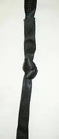
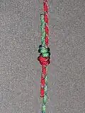
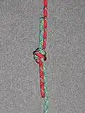
Beer knot: The Beer knot is often used in tubular webbing, usually for making slings.
Double fisherman knot (also known as Grapevine): The Grapevine knot is useful to tie together two ends of ropes. Ropes can be of unequal sizes. It is often used to tie both ends of the same rope together to form a circle.
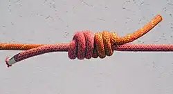
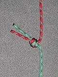
Overhand bend (also known as European death knot, Euro death knot, EDK): The Overhand bend is a simple and fast way to join two ropes, notably for rappelling. Can be very useful in situations where speed is critical to safety. It is similar to a water knot, but both bitter ends come out the same side of the knot.
Water knot (also known as Tape Knot, Double Overhand Bend, Ring Bend): The Water knot is useful to tie together two ends of ropes. Often used with webbing.
Binding
Strangle knot: The Strangle knot is a simple binding knot. It forms both sides of a Double fisherman’s knot, and is also used to back up loop knots and both ends of bends.
Hitches
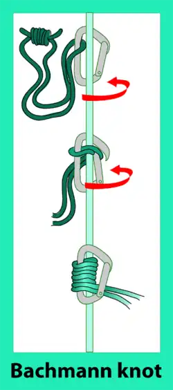
Bachmann knot: The Bachmann knot is useful when the friction hitch needs to be reset quickly/often or made to be self-tending as in crevasse and self-rescue.
Clove hitch: The Clove hitch is used in belay systems among other things.
Italian hitch (also known as Munter hitch, HMS): The Italian hitch is a simple knot, used by climbers and cavers as part of a life-lining or belay system. Its main use is as a friction device for controlling the rate of descent in belay systems.
Klemheist knot: The Klemheist knot is an alternative to the Prusik knot, useful when the climber is short of cord but has plenty of webbing.
Prusik: The Prusik is a knot used mainly for emergency use. Some carry between one and three cords specifically for prusiks. One can be used to quickly secure a person’s position to correct problems with equipment; two can be used as a method of ascending a rope.
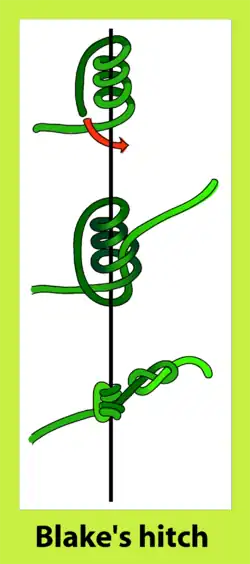
Blake’s hitch: Blake’s hitch is widely used in tree climbing applications. The knot can be slid up and down a line manually, but when loaded, it sticks securely.
Girth hitch: This hitch is commonly used to attach loops of runner to harnesses, bags, other kinds of equipment, and to natural features like rock knobs or brush/tree trunks for protection.
Loop Knots
Alpine butterfly knot: The Alpine Butterfly is a strong and secure loop knot. Allows load distribution in multiple directions. It can also be used to isolate a worn section of rope.
Figure-of-eight loop: The Figure-of-eight loop is considered strong and secure. Can be tied by taking a bight of rope and tying a figure-of-eight knot, or can be tied directly around/through objects by weaving back through the first figure eight knot (Figure-of-eight follow through), which is the standard method for attaching a rope to a climbing harness.[1]
Directional Figure-of-eight Loop: The Inline figure-of-eight loop is similar to a figure-of-eight loop but used to form a loop that will be loaded longitudinally in a line under tension. Particularly useful in rope tightening systems where the loop is established as a means to secure a pulley or carabiner onto the main line to reduce the amount of work needed to tighten the entire system. Similar to a trucker’s hitch.
Double bowline: The double bowline is commonly used by sport climbers who take multiple lead falls and then have trouble untying their figure eights.
Double Figure Eight Loop (also known as Bunny Ears): Used for equalising two anchors using the rope.
Yosemite bowline: Also called a bowline with a Yosemite finish, this is another way of tying the rope to the harness.
Stevedore knot (also known as Double figure eight): The Stevedore knot is tied at the end of a rope to prevent the end from unraveling, slipping through another knot, or passing back through a hole, block, or belay/rappel device. It is more bulky and less prone to jamming than the closely related figure-of-eight knot.
Overhand knot: The Overhand knot is a component of many knots used in climbing.
Monkey’s fist: The Monkey’s Fist is used to tie the end of a climbing rope into a tight ball so the rope can be thrown farther/easier.
This article is adapted from “List of climbing knots” on Wikipedia, written by its contributors, and used under CC BY-SA 4.0. Text on this page is available under the same licence. Source snapshot: Wikipedia via Kiwix, 2026-07-20.
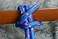
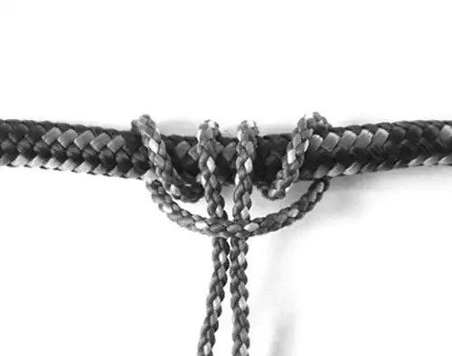
A binding knot is a knot that may be used to keep an object or multiple loose objects together, using a string or a rope that passes at least once around them. There are various binding knots, divided into two types. Friction knots are held in place by the friction between the windings of line. Knotted-ends knots are held in place by the two ends of the line being knotted together.
Stopping may be either a temporary whipping or seizing, the commonest variety consisting of a few round turns finished off with a reef knot. The purpose of a whipping is to prevent the end of a rope from fraying. A seizing holds several objects together.
↑Ashley, Clifford W. (1944). The Ashley Book of Knots, p.546. Doubleday. ISBN0-385-04025-3.
↑Ashley, Clifford W. (1944). The Ashley Book of Knots, #1208 (named: Whatnot). Doubleday. ISBN0-385-04025-3.
This article is adapted from “List of binding knots” on Wikipedia, written by its contributors, and used under CC BY-SA 4.0. Text on this page is available under the same licence. Source snapshot: Wikipedia via Kiwix, 2026-07-20.
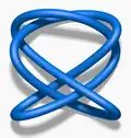
In knot theory, a Lissajous knot is a knot defined by parametric equations of the form
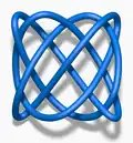
A Lissajous 821 knot
where , , and are integers and the phase shifts , , and may be any real numbers.[1]
The projection of a Lissajous knot onto any of the three coordinate planes is a Lissajous curve, and many of the properties of these knots are closely related to properties of Lissajous curves.
Replacing the cosine function in the parametrization by a triangle wave transforms every Lissajous
knot isotopically into a billiard curve inside a cube, the simplest case of so-called billiard knots.
Billiard knots can also be studied in other domains, for instance in a cylinder[2] or in a (flat) solid torus (Lissajous-toric knot).
Form
Because a knot cannot be self-intersecting, the three integers must be pairwise relatively prime, and none of the quantities
may be an integer multiple of pi. Moreover, by making a substitution of the form , one may assume that any of the three phase shifts , , is equal to zero.
Examples
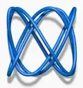
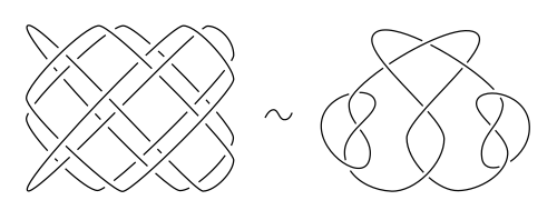
Here are some examples of Lissajous knots,[3] all of which have :
There are infinitely many different Lissajous knots,[4] and other examples with 10 or fewer crossings include the 74 knot, the 815 knot, the 101 knot, the 1035 knot, the 1058 knot, and the composite knot 52*#52,[1] as well as the 916 knot, 1076 knot, the 1099 knot, the 10122 knot, the 10144 knot, the granny knot, and the composite knot 52#52.[5] In addition, it is known that every twist knot with Arf invariant zero is a Lissajous knot.[6]
Symmetry
Lissajous knots are highly symmetric, though the type of symmetry depends on whether or not the numbers , , and are all odd.
Odd case
If , , and are all odd, then the point reflection across the origin is a symmetry of the Lissajous knot which preserves the knot orientation.
In general, a knot that has an orientation-preserving point reflection symmetry is known as strongly positive amphicheiral.[7] This is a fairly rare property: only seven prime knots with twelve or fewer crossings are strongly positive amphicheiral (1099, 10123, 12a427, 12a1019, 12a1105, 12a1202, 12n706).[8] Since this is so rare, ′most′ prime Lissajous knots lie in the even case.
Even case
If one of the frequencies (say ) is even, then the 180° rotation around the x-axis is a symmetry of the Lissajous knot. In general, a knot that has a symmetry of this type is called 2-periodic, so every even Lissajous knot must be 2-periodic.
Consequences
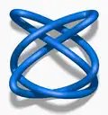
A Lissajous knot with three factors: ,
The symmetry of a Lissajous knot puts severe constraints on the Alexander polynomial. In the odd case, the Alexander
polynomial of the Lissajous knot must be a perfect square.[9] In the even case, the Alexander polynomial must be a perfect square modulo 2.[10] In addition, the Arf invariant of a Lissajous knot must be zero. It follows that:
12Bogle, M. G. V.; Hearst, J. E.; Jones, V. F. R.; Stoilov, L. (1994). “Lissajous knots”. Journal of Knot Theory and Its Ramifications. 3 (2): 121–140. doi:10.1142/S0218216594000095.
↑Hoste, Jim; Zirbel, Laura (2006). “Lissajous knots and knots with Lissajous projections”. arXiv:math.GT/0605632.
↑Przytycki, Jozef H. (2004). “Symmetric knots and billiard knots”. In Stasiak, A.; Katrich, V.; Kauffman, L. (eds.). Ideal Knots. Series on Knots and Everything. Vol.19. World Scientific. pp.374–414. arXiv:math/0405151. Bibcode:2004math……5151P.
↑See Lamm, Christoph (2023). “Strongly positive amphicheiral knots with doubly symmetric diagrams”. arXiv:2310.05106 [math.GT]. This article contains a complete list of prime strongly positive amphicheiral knots up to 16 crossings.
↑Hartley, R.; Kawauchi, A (1979). “Polynomials of amphicheiral knots”. Mathematische Annalen. 243: 63–70. doi:10.1007/bf01420207. S2CID120648664.
This article is adapted from “Lissajous knot” on Wikipedia, written by its contributors, and used under CC BY-SA 4.0. Text on this page is available under the same licence. Source snapshot: Wikipedia via Kiwix, 2026-07-20.
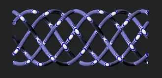
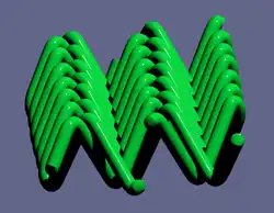
Lissajous-toric knot T(4,7,35) as a billiard knot, showing period 7
In braid form these knots can be defined in a square solid torus (i.e. the cube with identified top and bottom) as
.
The projection of this Lissajous-toric knot onto the x-y-plane is a Lissajous curve.
Replacing the sine and cosine functions in the parametrization by a triangle wave transforms a Lissajous-toric
knot isotopically into a billiard curve inside the solid torus. Because of this property Lissajous-toric knots are also called billiard knots in a solid torus.[2]
Lissajous-toric knots were first studied as billiard knots and they share many properties with billiard knots in a cylinder.[3]
They also occur in the analysis of singularities of minimal surfaces with branch points[4] and in the study of
the Three-body problem.[5]
The knots in the subfamily with , with an integer , are known as ′Lemniscate knots′.[6] Lemniscate knots have period and are fibred. The knot shown on the right is of this type (with ).
Properties
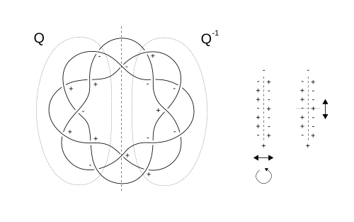
Symmetries of the Lissajous-toric knot T(3,8,7): symmetric union (vertical axis), rotation into mirror image and palindromic property within Q (horizontal axis)
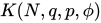
Lissajous-toric knots are denoted by . To ensure that the knot is traversed only once in the parametrization
the conditions are needed. In addition, singular values for the phase, leading to self-intersections, have to be excluded.
The isotopy class of Lissajous-toric knots surprisingly does not depend on the phase (up to mirroring).
If the distinction between a knot and its mirror image is not important, the notation can be used.
The properties of Lissajous-toric knots depend on whether and are coprime or . The main properties are:
Interchanging and :
(up to mirroring).
Ribbon property:
If and are coprime, is a symmetric union and therefore a ribbon knot.
Periodicity:
If , the Lissajous-toric knot has period and the factor knot is a ribbon knot.
Strongly positive amphicheirality:
If and have different parity, then is strongly positive amphicheiral.
Period 2:
If and are both odd, then has period 2 (for even ) or is freely 2-periodic (for odd ).
Example
The knot T(3,8,7), shown in the graphics, is a symmetric union and a ribbon knot (in fact, it is the composite knot ).
It is strongly positive amphicheiral: a rotation by maps the knot to its mirror image, keeping its orientation.
An additional horizontal symmetry occurs as a combination of the vertical symmetry and the rotation (′double palindromicity′ in Kin/Nakamura/Ogawa).
′Classification′ of billiard rooms
In the following table a systematic overview of the possibilities to build billiard rooms from the interval and the circle (interval with identified boundaries) is given:
In the case of Lissajous knots reflections at the boundaries occur in all of the three cube’s dimensions.
In the second case reflections occur in two dimensions and we have a uniform movement in the third dimension.
The third case is nearly equal to the usual movement on a torus, with an additional triangle wave movement in the first dimension.
References
↑See M. Soret and M. Ville: Lissajous-toric knots,
J. Knot Theory Ramifications 29, 2050003 (2020).
↑See C. Lamm:
Deformation of cylinder knots, 4th chapter of Ph.D. thesis, ‘Zylinder-Knoten und symmetrische Vereinigungen‘, Bonner Mathematische Schriften 321 (1999), available since 2012 as arXiv:1210.6639.
↑See C. Lamm and
D. Obermeyer: Billiard knots in a cylinder, J. Knot Theory Ramifications 8, 353–-366 (1999).
This article is adapted from “Lissajous-toric knot” on Wikipedia, written by its contributors, and used under CC BY-SA 4.0. Text on this page is available under the same licence. Source snapshot: Wikipedia via Kiwix, 2026-07-20.
In topological graph theory, a mathematical discipline, a linkless embedding of an undirected graph is an embedding of the graph into three-dimensional Euclidean space in such a way that no two cycles of the graph are linked. A flat embedding is an embedding with the property that every cycle is the boundary of a topological disk whose interior is disjoint from the graph. A linklessly embeddable graph is a graph that has a linkless or flat embedding; these graphs form a three-dimensional analogue of the planar graphs.[1] Complementarily, an intrinsically linked graph is a graph that does not have a linkless embedding.
Flat embeddings are automatically linkless, but not vice versa.[2] The complete graph K6, the Petersen graph, and the other five graphs in the Petersen family do not have linkless embeddings.[1] Every graph minor of a linklessly embeddable graph is again linklessly embeddable,[3] as is every graph that can be reached from a linklessly embeddable graph by YΔ- and ΔY-transformations.[2] The linklessly embeddable graphs have the Petersen family graphs as their forbidden minors,[4] and include the planar graphs and apex graphs.[2] They may be recognized, and a flat embedding may be constructed for them, in O(n2).[5]
When the circle is mapped to three-dimensional Euclidean space by an injective function (a continuous function that does not map two different points of the circle to the same point of space), its image is a closed curve.
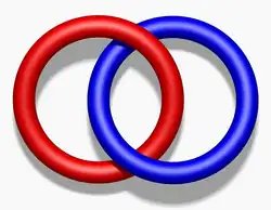
Two disjoint closed curves that both lie on the same plane are unlinked, and more generally a pair of disjoint closed curves is said to be unlinked when there is a continuous deformation of space that moves them both onto the same plane, without either curve passing through the other or through itself. If there is no such continuous motion, the two curves are said to be linked. For example, the Hopf link is formed by two circles that each pass through the disk spanned by the other. It forms the simplest example of a pair of linked curves, but it is possible for curves to be linked in other more complicated ways. If two curves are not linked, then it is possible to find a topological disk in space, having the first curve as its boundary and disjoint from the second curve. Conversely if such a disk exists then the curves are necessarily unlinked.
The linking number of two closed curves in three-dimensional space is a topological invariant of the curves: it is a number, defined from the curves in any of several equivalent ways, that does not change if the curves are moved continuously without passing through each other. The version of the linking number used for defining linkless embeddings of graphs is found by projecting the embedding onto the plane and counting the number of crossings of the projected embedding in which the first curve passes over the second one, modulo 2.[2] The projection must be “regular”, meaning that no two vertices project to the same point, no vertex projects to the interior of an edge, and at every point of the projection where the projections of two edges intersect, they cross transversally; with this restriction, any two projections lead to the same linking number.
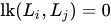
The linking number of the unlink is zero, and therefore, if a pair of curves has nonzero linking number, the two curves must be linked. However, there are examples of curves that are linked but that have zero linking number, such as the Whitehead link.
An embedding of a graph into three-dimensional space consists of a mapping from the vertices of the graph to points in space, and from the edges of the graph to curves in space, such that each endpoint of each edge is mapped to an endpoint of the corresponding curve, and such that the curves for two different edges do not intersect except at a common endpoint of the edges.
Any finite graph has a finite (though perhaps exponential) number of distinct simple cycles, and if the graph is embedded into three-dimensional space then each of these cycles forms a simple closed curve. One may compute the linking number of each disjoint pair of curves formed in this way; if all pairs of cycles have zero linking number, the embedding is said to be linkless.[6]
In some cases, a graph may be embedded in space in such a way that, for each cycle in the graph, one can find a disk bounded by that cycle that does not cross any other feature of the graph. In this case, the cycle must be unlinked from all the other cycles disjoint from it in the graph. The embedding is said to be flat if every cycle bounds a disk in this way.[7] A flat embedding is necessarily linkless, but there may exist linkless embeddings that are not flat: for instance, if G is a graph formed by two disjoint cycles, and it is embedded to form the Whitehead link, then the embedding is linkless but not flat.
A graph is said to be intrinsically linked if, no matter how it is embedded, the embedding is always linked. Although linkless and flat embeddings are not the same, the graphs that have linkless embeddings are the same as the graphs that have flat embeddings.[8]
Examples and counterexamples
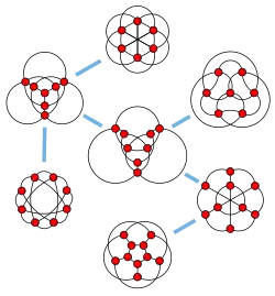
The Petersen family.
As Sachs (1983) showed, each of the seven graphs of the Petersen family is intrinsically linked: no matter how each of these graphs is embedded in space, they have two cycles that are linked to each other. These graphs include the complete graph K6, the Petersen graph, the graph formed by removing an edge from the complete bipartite graph K4,4, and the complete tripartite graph K3,3,1.
Every planar graph has a flat and linkless embedding: simply embed the graph into a plane and embed the plane into space. If a graph is planar, this is the only way to embed it flatly and linklessly into space: every flat embedding can be continuously deformed to lie on a flat plane. And conversely, every nonplanar linkless graph has multiple linkless embeddings.[2]
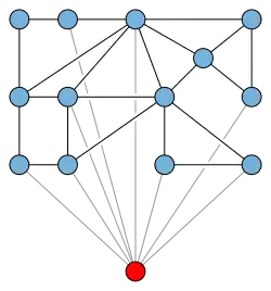
An apex graph. If the planar part of the graph is embedded on a flat plane in space, and the apex vertex is placed above the plane and connected to it by straight line segments, the resulting embedding is flat.
An apex graph, formed by adding a single vertex to a planar graph, also has a flat and linkless embedding: embed the planar part of the graph on a plane, place the apex above the plane, and draw the edges from the apex to its neighbors as line segments. Any closed curve within the plane bounds a disk below the plane that does not pass through any other graph feature, and any closed curve through the apex bounds a disk above the plane that does not pass through any other graph feature.[2]
If a graph has a linkless or flat embedding, then modifying the graph by subdividing or unsubdividing its edges, adding or removing multiple edges between the same pair of points, and performing YΔ- and ΔY-transformations that replace a degree-three vertex by a triangle connecting its three neighbors or the reverse all preserve flatness and linklessness.[2] In particular, in a cubic planar graph (one in which all vertices have exactly three neighbors, such as the cube) it is possible to make duplicates of any independent set of vertices by performing a YΔ-transformation, adding multiple copies of the resulting triangle edges, and then performing the reverse ΔY-transformations.
Characterization and recognition
If a graph G has a linkless or flat embedding, then every minor of G (a graph formed by contraction of edges and deletion of edges and vertices) also has a linkless or flat embedding. Deletions cannot destroy the flatness of an embedding, and a contraction can be performed by leaving one endpoint of the contracted edge in place and rerouting all the edges incident to the other endpoint along the path of the contracted edge. Therefore, by the Robertson–Seymour theorem, the linklessly embeddable graphs have a forbidden graph characterization as the graphs that do not contain any of a finite set of minors.[3]
The set of forbidden minors for the linklessly embeddable graphs was identified by Sachs (1983): the seven graphs of the Petersen family are all minor-minimal intrinsically linked graphs. However, Sachs was unable to prove that these were the only minimal linked graphs, and this was finally accomplished by Robertson, Seymour & Thomas (1995).
The forbidden minor characterization of linkless graphs leads to a polynomial time algorithm for their recognition, but not for actually constructing an embedding. Kawarabayashi, Kreutzer & Mohar (2010) described a linear time algorithm that tests whether a graph is linklessly embeddable and, if so, constructs a flat embedding of the graph. Their algorithm finds large planar subgraphs within the given graph such that, if a linkless embedding exists, it has to respect the planar embedding of the subgraph. By repeatedly simplifying the graph whenever such a subgraph is found, they reduce the problem to one in which the remaining graph has bounded treewidth, at which point it can be solved by dynamic programming.
The problem of efficiently testing whether a given embedding is flat or linkless was posed by Robertson, Seymour & Thomas (1993a). It remains unsolved, and is equivalent in complexity to unknotting problem, the problem of testing whether a single curve in space is unknotted.[5] Testing unknottedness (and therefore, also, testing linklessness of an embedding) is known to be in NP but is not known to be NP-complete.[9]
Related families of graphs
Graphs with small Colin de Verdière invariant
The Colin de Verdière graph invariant is an integer defined for any graph using algebraic graph theory. The graphs with Colin de Verdière graph invariant at most μ, for any fixed constant μ, form a minor-closed family, and the first few of these are well-known: the graphs with μ ≤ 1 are the linear forests (disjoint unions of paths), the graphs with μ ≤ 2 are the outerplanar graphs, and the graphs with μ ≤ 3 are the planar graphs. As Robertson, Seymour & Thomas (1993a) conjectured and Lovász & Schrijver (1998) proved, the graphs with μ ≤ 4 are exactly the linklessly embeddable graphs.
Apex graphs
A linkless apex graph that is not YΔY reducible.
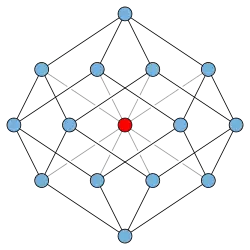
The planar graphs and the apex graphs are linklessly embeddable, as are the graphs obtained by YΔ- and ΔY-transformations from these graphs.[2] The YΔY reducible graphs are the graphs that can be reduced to a single vertex by YΔ- and ΔY-transformations, removal of isolated vertices and degree-one vertices, and compression of degree-two vertices; they are also minor-closed, and include all planar graphs. However, there exist linkless graphs that are not YΔY reducible, such as the apex graph formed by connecting an apex vertex to every degree-three vertex of a rhombic dodecahedron.[10] There also exist linkless graphs that cannot be transformed into an apex graph by YΔ- and ΔY-transformation, removal of isolated vertices and degree-one vertices, and compression of degree-two vertices: for instance, the ten-vertex crown graph has a linkless embedding, but cannot be transformed into an apex graph in this way.[2]
Knotless graphs
A closed curve forming a trefoil, the simplest nontrivial knot.
Related to the concept of linkless embedding is the concept of knotless embedding, an embedding of a graph in such a way that none of its simple cycles form a nontrivial knot. The graphs that do not have knotless embeddings (that is, they are intrinsically knotted) include K7 and K3,3,1,1.[11] However, there also exist minimal forbidden minors for knotless embedding that are not formed (as these two graphs are) by adding one vertex to an intrinsically linked graph, but the list of these is unknown.[12]
One may also define graph families by the presence or absence of more complex knots and links in their embeddings,[13] or by linkless embedding in three-dimensional manifolds other than Euclidean space.[14]Flapan, Naimi & Pommersheim (2001) define a graph embedding to be triple linked if there are three cycles no one of which can be separated from the other two; they show that K9 is not intrinsically triple linked, but K10 is.[15] More generally, one can define an n-linked embedding for any n to be an embedding that contains an n-component link that cannot be separated by a topological sphere into two separated parts; minor-minimal graphs that are intrinsically n-linked are known for all n.[16]
Directed graphs
A directed graph is said to be intrinsically linked if it contains a nontrivial link consisting of a pair of consistently oriented directed cycles in every spatial embedding. In contrast to undirected graphs, edge contraction and ∆−Y operations do not necessarily preserve linkless embeddability.[17]
History
The question of whether K6 has a linkless or flat embedding was posed within the topology research community in the early 1970s by Bothe (1973). Linkless embeddings were brought to the attention of the graph theory community by HorstSachs(1983), who posed several related problems including the problem of finding a forbidden graph characterization of the graphs with linkless and flat embeddings; Sachs showed that the seven graphs of the Petersen family (including K6) do not have such embeddings. As Nešetřil & Thomas (1985) observed, linklessly embeddable graphs are closed under graph minors, from which it follows by the Robertson–Seymour theorem that a forbidden graph characterization exists. The proof of the existence of a finite set of obstruction graphs does not lead to an explicit description of this set of forbidden minors, but it follows from Sachs’ results that the seven graphs of the Petersen family belong to the set. These problems were finally settled by Robertson, Seymour & Thomas (1995),[18] who showed that the seven graphs of the Petersen family are the only minimal forbidden minors for these graphs. Therefore, linklessly embeddable graphs and flat embeddable graphs are both the same set of graphs, and are both the same as the graphs that have no Petersen family minor.
Sachs (1983) also asked for bounds on the number of edges and the chromatic number of linkless embeddable graphs. The number of edges in an n-vertex linkless graph is at most 4n−10: maximal apex graphs with n>4 have exactly this many edges,[1] and Mader (1968) proved a matching upper bound on the more general class of K6-minor-free graphs. Nešetřil & Thomas (1985) observed that Sachs’ question about the chromatic number would be resolved by a proof of Hadwiger’s conjecture that any k-chromatic graph has as a minor a k-vertex complete graph. The proof by Robertson, Seymour & Thomas (1993c) of the case k=6 of Hadwiger’s conjecture is sufficient to settle Sachs’ question: the linkless graphs can be colored with at most five colors, as any 6-chromatic graph contains a K6 minor and is not linkless, and there exist linkless graphs such as K5 that require five colors. The snark theorem implies that every cubic linklessly embeddable graph is 3-edge-colorable.
Linkless embeddings started being studied within the algorithms research community in the late 1980s through the works of Fellows & Langston (1988) and Motwani, Raghunathan & Saran (1988). Algorithmically, the problem of recognizing linkless and flat embeddable graphs was settled once the forbidden minor characterization was proven: an algorithm of Robertson & Seymour (1995) can be used to test in polynomial time whether a given graph contains any of the seven forbidden minors.[19] This method does not construct linkless or flat embeddings when they exist, but an algorithm that does construct an embedding was developed by van der Holst (2009), and a more efficient linear time algorithm was found by Kawarabayashi, Kreutzer & Mohar (2010).
A final question of Sachs (1983) on the possibility of an analogue of Fáry’s theorem for linkless graphs appears not to have been answered: when does the existence of a linkless or flat embedding with curved or piecewise linear edges imply the existence of a linkless or flat embedding in which the edges are straight line segments?
↑The application of the Robertson–Seymour algorithm to this problem was noted by Fellows & Langston (1988).
References
Böhme, Thomas (1990), “On spatial representations of graphs”, in Bodendieck, Rainer (ed.), Contemporary Methods in Graph Theory: In honor of Prof. Dr. Klaus Wagner, Mannheim: Bibliographisches Institut, Wissenschaftsverlag, pp.151–167, ISBN978-3-411-14301-6. As cited by Robertson, Seymour & Thomas (1993a).
Bothe, H.-G. (1973), “Problem P855”, Colloquium Mathematicum, 28: 163, New Scottish Book, Problem 876, 20.5.1972. As cited by Sachs (1983).
Conway, John H.; Gordon, Cameron McA. (1983), “Knots and links in spatial graphs”, Journal of Graph Theory, 7 (4): 445–453, doi:10.1002/jgt.3190070410.
Fellows, Michael R.; Langston, Michael A. (1988), “Nonconstructive tools for proving polynomial-time decidability”, Journal of the ACM, 35 (3): 727–739, doi:10.1145/44483.44491.
Flapan, Erica; Howards, Hugh; Lawrence, Don; Mellor, Blake (2006), “Intrinsic linking and knotting of graphs in arbitrary 3–manifolds”, Algebraic & Geometric Topology, 6 (3): 1025–1035, arXiv:math/0508004, doi:10.2140/agt.2006.6.1025.
Fleming, Thomas; Diesl, Alexander (2005), “Intrinsically linked graphs and even linking number”, Algebraic & Geometric Topology, 5 (4): 1419–1432, arXiv:math/0511133, doi:10.2140/agt.2005.5.1419.
Foisy, Joel (2002), “Intrinsically knotted graphs”, Journal of Graph Theory, 39 (3): 178–187, doi:10.1002/jgt.10017.
Foisy, Joel (2003), “A newly recognized intrinsically knotted graph”, Journal of Graph Theory, 43 (3): 199–209, doi:10.1002/jgt.10114.
Hass, Joel; Lagarias, Jeffrey C.; Pippenger, Nicholas (1999), “The computational complexity of knot and link problems”, Journal of the ACM, 46 (2): 185–211, arXiv:math/9807016, doi:10.1145/301970.301971.
van der Holst, Hein (2009), “A polynomial-time algorithm to find a linkless embedding of a graph”, Journal of Combinatorial Theory, Series B, 99 (2): 512–530, doi:10.1016/j.jctb.2008.10.002.
Kawarabayashi, Ken-ichi; Kreutzer, Stephan; Mohar, Bojan (2010), “Linkless and flat embeddings in 3-space and the unknot problem”, Proc. ACM Symposium on Computational Geometry (SoCG ’10), pp.97–106, doi:10.1145/1810959.1810975, ISBN978-1-4503-0016-2.
Lovász, László; Schrijver, Alexander (1998), “A Borsuk theorem for antipodal links and a spectral characterization of linklessly embeddable graphs”, Proceedings of the American Mathematical Society, 126 (5): 1275–1285, doi:10.1090/S0002-9939-98-04244-0.
Mader, W. (1968), “Homomorphiesätze für Graphen”, Mathematische Annalen, 178 (2): 154–168, doi:10.1007/BF01350657.
Motwani, Rajeev; Raghunathan, Arvind; Saran, Huzur (1988), “Constructive results from graph minors: linkless embeddings”, Proc. 29th IEEE Symposium on Foundations of Computer Science (FOCS ’88), pp.398–409, doi:10.1109/SFCS.1988.21956, ISBN0-8186-0877-3.
Robertson, Neil; Seymour, Paul (1995), “Graph Minors. XIII. The disjoint paths problem”, Journal of Combinatorial Theory, Series B, 63 (1): 65–110, doi:10.1006/jctb.1995.1006.
Robertson, Neil; Seymour, P. D.; Thomas, Robin (1993b), “Linkless embeddings of graphs in 3-space”, Bulletin of the American Mathematical Society, 28 (1): 84–89, arXiv:math/9301216, doi:10.1090/S0273-0979-1993-00335-5, MR1164063.
Robertson, Neil; Seymour, P. D.; Thomas, Robin (1995), “Sachs’ linkless embedding conjecture”, Journal of Combinatorial Theory, Series B, 64 (2): 185–227, doi:10.1006/jctb.1995.1032.
Sachs, Horst (1983), “On a spatial analogue of Kuratowski’s Theorem on planar graphs – an open problem”, in Horowiecki, M.; Kennedy, J. W.; Sysło, M. M. (eds.), Graph Theory: Proceedings of a Conference held in Łagów, Poland, February 10–13, 1981, Lecture Notes in Mathematics, vol.1018, Springer-Verlag, pp.230–241, doi:10.1007/BFb0071633, ISBN978-3-540-12687-4.
Saran, Huzur (1989), Constructive Results in Graph Minors: Linkless Embeddings, Ph.D. thesis, University of California, Berkeley.
Truemper, Klaus (1992), Matroid Decomposition(PDF), Academic Press, pp.100–101, archived from the original(PDF) on 2017-08-29, retrieved 2010-08-05.
Further reading
Ramírez Alfonsín, J. L. (2005), “Knots and links in spatial graphs: a survey”, Discrete Mathematics, 302 (1–3): 225–242, doi:10.1016/j.disc.2004.07.035.
This article is adapted from “Linkless embedding” on Wikipedia, written by its contributors, and used under CC BY-SA 4.0. Text on this page is available under the same licence. Source snapshot: Wikipedia via Kiwix, 2026-07-20.
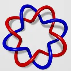
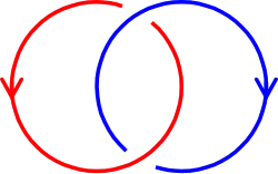
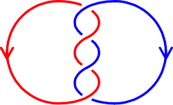
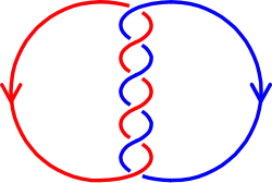
The two curves of this (2, 8)-torus link have linking number four.
In mathematics, the linking number is a numerical invariant that describes the linking of two closed curves in three-dimensional space. Intuitively, the linking number represents the number of times that each curve winds around the other. In Euclidean space, the linking number is always an integer, but may be positive or negative depending on the orientation of the two curves (this is not true for curves in most 3-manifolds, where linking numbers can also be fractions or just not exist at all).
The linking number was introduced by Gauss in the form of the linking integral. It is an important object of study in knot theory, algebraic topology, and differential geometry, and has numerous applications in mathematics and science, including quantum mechanics, electromagnetism, and the study of DNA supercoiling.
Definition
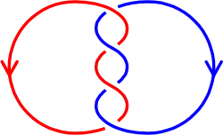
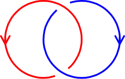
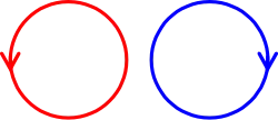
Any two closed curves in space, if allowed to pass through themselves but not each other, can be moved into exactly one of the following standard positions. This determines the linking number:
⋯
linking number −2
linking number −1
linking number 0
⋯
linking number 1
linking number 2
linking number 3
Each curve may pass through itself during this motion, but the two curves must remain separated throughout. This is formalized as regular homotopy, which further requires that each curve be an immersion, not just any map. However, this added condition does not change the definition of linking number (it does not matter if the curves are required to always be immersions or not), which is an example of an h-principle (homotopy-principle), meaning that geometry reduces to topology.
Proof
This fact (that the linking number is the only invariant) is most easily proven by placing one circle in standard position, and then showing that linking number is the only invariant of the other circle. In detail:
A single curve is regular homotopic to a standard circle (any knot can be unknotted if the curve is allowed to pass through itself). The fact that it is homotopic is clear, since 3-space is contractible and thus all maps into it are homotopic, though the fact that this can be done through immersions requires some geometric argument.
The complement of a standard circle is homeomorphic to a solid torus with a point removed (this can be seen by interpreting 3-space as the 3-sphere with the point at infinity removed, and the 3-sphere as two solid tori glued along the boundary), or the complement can be analyzed directly.
The fundamental group of 3-space minus a circle is the integers, corresponding to linking number. This can be seen via the Seifert–Van Kampen theorem (either adding the point at infinity to get a solid torus, or adding the circle to get 3-space, allows one to compute the fundamental group of the desired space).
Thus homotopy classes of a curve in 3-space minus a circle are determined by linking number.
It is also true that regular homotopy classes are determined by linking number, which requires additional geometric argument.
Computing the linking number
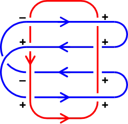
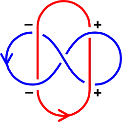
With six positive crossings and two negative crossings, these curves have linking number two.
There is an algorithm to compute the linking number of two curves from a link diagram. Label each crossing as positive or negative, according to the following rule:[1]
The total number of positive crossings minus the total number of negative crossings is equal to twice the linking number. That is:
where n1, n2, n3, n4 represent the number of crossings of each of the four types. The two sums and are always equal,[2] which leads to the following alternative formula
The formula involves only the undercrossings of the blue curve by the red, while involves only the overcrossings.
Properties and examples
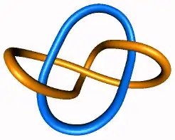
The two curves of the Whitehead link have linking number zero.
Any two unlinked curves have linking number zero. However, two curves with linking number zero may still be linked (e.g. the Whitehead link).
Reversing the orientation of either of the curves negates the linking number, while reversing the orientation of both curves leaves it unchanged.
The linking number is chiral: taking the mirror image of link negates the linking number. The convention for positive linking number is based on a right-hand rule.
The winding number of an oriented curve in the x–y plane is equal to its linking number with the z-axis (thinking of the z-axis as a closed curve in the 3-sphere).
More generally, if either of the curves is simple, then the first homology group of its complement is isomorphic to Z. In this case, the linking number is determined by the homology class of the other curve.
In physics, the linking number is an example of a topological quantum number.
Gauss’s integral definition
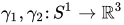
Given two non-intersecting differentiable curves , define the Gauss map from the torus to the sphere by
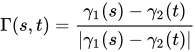
Pick a point in the unit sphere, v, so that orthogonal projection of the link to the plane perpendicular to v gives a link diagram. Observe that a point (s, t) that goes to v under the Gauss map corresponds to a crossing in the link diagram where is over . Also, a neighborhood of (s, t) is mapped under the Gauss map to a neighborhood of v preserving or reversing orientation depending on the sign of the crossing. Thus in order to compute the linking number of the diagram corresponding to v it suffices to count the signed number of times the Gauss map covers v. Since v is a regular value, this is precisely the degree of the Gauss map (i.e. the signed number of times that the image of Γ covers the sphere). Isotopy invariance of the linking number is automatically obtained as the degree is invariant under homotopic maps. Any other regular value would give the same number, so the linking number doesn’t depend on any particular link diagram.
This formulation of the linking number of γ1 and γ2 enables an explicit formula as a double line integral, the Gauss linking integral:
This integral computes the total signed area of the image of the Gauss map (the integrand being the Jacobian of Γ) and then divides by the area of the sphere (which is 4π).
In quantum field theory
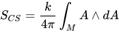
In quantum field theory, Gauss’s integral definition arises when computing the expectation value of the Wilson loop observable in Chern–Simons gauge theory. Explicitly, the abelian Chern–Simons action for a gauge potential one-form on a three-manifold is given by
We are interested in doing the Feynman path integral for Chern–Simons in :
Here, is the antisymmetric symbol. Since the theory is just Gaussian, no ultraviolet regularization or renormalization is needed. Therefore, the topological invariance of right hand side ensures that the result of the path integral will be a topological invariant. The only thing left to do is provide an overall normalization factor, and a natural choice will present itself. Since the theory is Gaussian and abelian, the path integral can be done simply by solving the theory classically and substituting for .
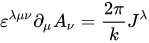
The classical equations of motion are
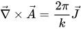
Here, we have coupled the Chern–Simons field to a source with a term in the Lagrangian. Obviously, by substituting the appropriate , we can get back the Wilson loops. Since we are in 3 dimensions, we can rewrite the equations of motion in a more familiar notation:
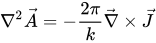
Taking the curl of both sides and choosing Lorenz gauge , the equations become
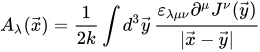
From electrostatics, the solution is
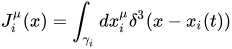
The path integral for arbitrary is now easily done by substituting this into the Chern–Simons action to get an effective action for the field. To get the path integral for the Wilson loops, we substitute for a source describing two particles moving in closed loops, i.e. , with
Since the effective action is quadratic in , it is clear that there will be terms describing the self-interaction of the particles, and these are uninteresting since they would be there even in the presence of just one loop. Therefore, we normalize the path integral by a factor precisely cancelling these terms. Going through the algebra, we obtain
where
which is simply Gauss’s linking integral. This is the simplest example of a topological quantum field theory, where the path integral computes topological invariants. This also served as a hint that the nonabelian variant of Chern–Simons theory computes other knot invariants, and it was shown explicitly by Edward Witten that the nonabelian theory gives the invariant known as the Jones polynomial. [3]
The Chern-Simons gauge theory lives in 3 spacetime dimensions. More generally, there exists higher dimensional topological quantum field theories. There exists more complicated multi-loop/string-braiding statistics of 4-dimensional gauge theories captured by the link invariants of exotic topological quantum field theories in 4 spacetime dimensions. [4]
Generalizations
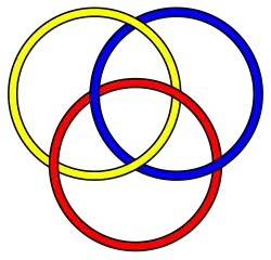
The Milnor invariants generalize linking number to links with three or more components, allowing one to prove that the Borromean rings are linked, though any two components have linking number 0.
Just as closed curves can be linked in three dimensions, any two closed manifolds of dimensions m and n may be linked in a Euclidean space of dimension . Any such link has an associated Gauss map, whose degree is a generalization of the linking number.
Any framed knot has a self-linking number obtained by computing the linking number of the knot C with a new curve obtained by slightly moving the points of C along the framing vectors. The self-linking number obtained by moving vertically (along the blackboard framing) is known as Kauffman’s self-linking number.
The linking number is defined for two linked circles; given three or more circles, one can define the Milnor invariants, which are a numerical invariant generalizing linking number.
In algebraic topology, the cup product is a far-reaching algebraic generalization of the linking number, with the Massey products being the algebraic analogs for the Milnor invariants.
A linkless embedding of an undirected graph is an embedding into three-dimensional space such that every two cycles have zero linking number. The graphs that have a linkless embedding have a forbidden minor characterization as the graphs with no Petersen family minor.
See also
Differentiable curve– Study of curves from a differential point of view
Hopf invariant– Homotopy invariant of maps between n-spheres
↑This is the same labeling used to compute the writhe of a knot, though in this case we only label crossings that involve both curves of the link.
↑This follows from the Jordan curve theorem if either curve is simple. For example, if the blue curve is simple, then n1+n3 and n2+n4 represent the number of times that the red curve crosses in and out of the region bounded by the blue curve.
This article is adapted from “Linking number” on Wikipedia, written by its contributors, and used under CC BY-SA 4.0. Text on this page is available under the same licence. Source snapshot: Wikipedia via Kiwix, 2026-07-20.
In knot theory, an area of mathematics, the link group of a link is an analog of the knot group of a knot. They were described by John Milnor in his Ph.D. thesis, (Milnor 1954). Notably, the link group is not in general the fundamental group of the link complement.
Definition
The Whitehead link is link homotopic to the unlink, but not isotopic to the unlink.
The link group of an n-component link is essentially the set of (n+1)-component links extending this link, up to link homotopy. In other words, each component of the extended link is allowed to move through regular homotopy (homotopy through immersions), knotting or unknotting itself, but is not allowed to move through other components. This is a weaker condition than isotopy: for example, the Whitehead link has linking number0, and thus is link homotopic to the unlink, but it is not isotopic to the unlink.
The link group is not the fundamental group of the link complement, since the components of the link are allowed to move through themselves, though not each other, but thus is a quotient group of the link complement’s fundamental group, since one can start with elements of the fundamental group, and then by knotting or unknotting components, some of these elements may become equivalent to each other.
Examples
The link group of the n-component unlink is the free group on n generators, , as the link group of a single link is the knot group of the unknot, which is the integers, and the link group of an unlinked union is the free product of the link groups of the components.
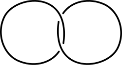
The link group of the Hopf link, the simplest non-trivial link – two circles, linked once – is the free abelian group on two generators, Note that the link group of two unlinked circles is the free nonabelian group on two generators, of which the free abelian group on two generators is a quotient. In this case the link group is the fundamental group of the link complement, as the link complement deformation retracts onto a torus.
The Whitehead link is link homotopic to the unlink – though it is not isotopic to the unlink – and thus has link group the free group on two generators.
Milnor invariants
Milnor defined invariants of a link (functions on the link group) in (Milnor 1954), using the character which have thus come to be called “Milnor’s μ-bar invariants”, or simply the “Milnor invariants”. For each k, there is a k-ary function which defines invariants according to which k of the links one selects, in which order.
Milnor’s invariants can be related to Massey products on the link complement (the complement of the link); this was suggested in (Stallings 1965), and made precise in (Turaev 1976) and (Porter 1980).
As with Massey products, the Milnor invariants of length k+1 are defined if all Milnor invariants of length less than or equal to k vanish. The first (2-fold) Milnor invariant is simply the linking number (just as the 2-fold Massey product is the cup product, which is dual to intersection), while the 3-fold Milnor invariant measures whether 3 pairwise unlinked circles are Borromean rings, and if so, in some sense, how many times (that is to say, the Borromean rings have a Milnor 3-fold invariant of 1 or –1, depending on order, but other 3-element links can have an invariant of 2 or more, just as linking numbers can be greater than 1).
Another definition is the following: consider a link . Suppose that for and . Pick any Seifert surfaces for the respective link components, say, , such that for all . Then the Milnor 3-fold invariant equals minus the number of intersection points in counting with signs; (Cochran 1990).
Milnor invariants can also be defined if the lower order invariants do not vanish, but then there is an indeterminacy, which depends on the values of the lower order invariants. This indeterminacy can be understood geometrically as the indeterminacy in expressing a link as a closed string link, as discussed below (it can also be seen algebraically as the indeterminacy of Massey products if lower order Massey products do not vanish).
Milnor invariants can be considered as invariants of string links, in which case they are universally defined, and the indeterminacy of the Milnor invariant of a link is precisely due to the multiple ways that a given links can be cut into a string link; this allows the classification of links up to link homotopy, as in (Habegger & Lin 1990). Viewed from this point of view, Milnor invariants are finite type invariants, and in fact they (and their products) are the only rational finite type concordance invariants of string links; (Habegger & Masbaum 2000).
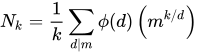
The number of linearly independent Milnor invariants of length for m-component links is , where is the number of basic commutators of length k in the free Lie algebra on m generators, namely:
,
where is the Möbius function; see for instance (Orr 1989). This number grows on the order of .
Habegger, Nathan; Lin, Xiao Song (1990), “The classification of links up to homotopy”, Journal of the American Mathematical Society, 2, 3 (2), American Mathematical Society: 389–419, doi:10.2307/1990959, JSTOR1990959
Habegger, Nathan; Masbaum, Gregor (2000), “The Kontsevich integral and Milnor’s invariants”, Topology, 39 (6): 1253–1289, doi:10.1016/S0040-9383(99)00041-5, MR1783857
Milnor, John (March 1954), “Link groups”, Annals of Mathematics, 59 (2), Annals of Mathematics: 177–195, doi:10.2307/1969685, JSTOR1969685, MR0071020
Orr, Kent E. (1989), “Homotopy invariants of links”, Inventiones Mathematicae, 95 (2): 379–394, doi:10.1007/BF01393902, MR0974908, S2CID120916814
Porter, Richard D. (1980), “Milnor’s μ-invariants and Massey products”, Transactions of the American Mathematical Society, 257 (1), American Mathematical Society: 39–71, doi:10.2307/1998124, JSTOR1998124, MR0549154
Stallings, John R. (1965), “Homology and central series of groups”, Journal of Algebra, 2 (2): 170–181, doi:10.1016/0021-8693(65)90017-7, MR0175956
Turaev, Vladimir G. (1976), “The Milnor invariants and Massey products”, Zap. Naučn. Sem. Leningrad. Otdel. Mat. Inst. Steklov. (LOMI), Studies in Topology-II, 66: 189–203, MR0451251
This article is adapted from “Link group” on Wikipedia, written by its contributors, and used under CC BY-SA 4.0. Text on this page is available under the same licence. Source snapshot: Wikipedia via Kiwix, 2026-07-20.
In mathematics, two links and are concordant if there exists an embedding such that and .
By its nature, link concordance is an equivalence relation. It is weaker than isotopy, and stronger than homotopy: isotopy implies concordance implies homotopy. A link is a slice link if it is concordant to the unlink.
Concordance invariants
A function of a link that is invariant under concordance is called a concordance invariant.
The linking number of any two components of a link is one of the most elementary concordance invariants. The signature of a knot is also a concordance invariant. A subtler concordance invariant are the Milnor invariants, and in fact all rational finite type concordance invariants are Milnor invariants and their products,[1] though non-finite type concordance invariants exist.
Higher dimensions
One can analogously define concordance for any two submanifolds . In this case one considers two submanifolds concordant if there is a cobordism between them in i.e., if there is a manifold with boundary whose boundary consists of and
This higher-dimensional concordance is a relative form of cobordism – it requires two submanifolds to be not just abstractly cobordant, but “cobordant in N“.
↑Habegger, Nathan; Masbaum, Gregor (2000), “The Kontsevich integral and Milnor’s invariants”, Topology, 39 (6): 1253–1289, doi:10.1016/S0040-9383(99)00041-5
Further reading
J. Hillman, Algebraic invariants of links. Series on Knots and everything. Vol 32. World Scientific.
Livingston, Charles, A survey of classical knot concordance, in: Handbook of knot theory, pp 319–347, Elsevier, Amsterdam, 2005. MR2179265 ISBN0-444-51452-X
This article is adapted from “Link concordance” on Wikipedia, written by its contributors, and used under CC BY-SA 4.0. Text on this page is available under the same licence. Source snapshot: Wikipedia via Kiwix, 2026-07-20.





















![{\displaystyle [-1,1]^{3}}](/wp-content/uploads/wiki-images/98ff687f83fe9fc6244d40b9cb2f905a70b669a0-a7d03650.svg)
![{\displaystyle x(t)=\sin 2\pi qt,\qquad y(t)=\cos 2\pi p(t+\phi ),\qquad z(t)=2(Nt-\lfloor Nt\rfloor )-1,\qquad t\in [0,1]}](/wp-content/uploads/wiki-images/2c54fe71777efccf873b68da4df8b1fcc5194fa9-e4c96a4c.svg)








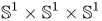
![{\displaystyle [-1,1]^{2}\times \mathbb {S} ^{1}}](/wp-content/uploads/wiki-images/347fb1274b11bc218afba8c30a88583d116fd76b-1fe59a64.svg)
![{\displaystyle [-1,1]\times \mathbb {S} ^{1}\times \mathbb {S} ^{1}}](/wp-content/uploads/wiki-images/8591b9ef82b90649d00841d8dcb4f69925d1aa4e-710e1a9a.svg)












![{\displaystyle {\begin{aligned}\operatorname {link} (\gamma _{1},\gamma _{2})&={\frac {1}{4\pi }}\oint _{\gamma _{1}}\oint _{\gamma _{2}}{\frac {\mathbf {r} _{1}-\mathbf {r} _{2}}{|\mathbf {r} _{1}-\mathbf {r} _{2}|^{3}}}\cdot (d\mathbf {r} _{1}\times d\mathbf {r} _{2})\\[4pt]&={\frac {1}{4\pi }}\int _{S^{1}\times S^{1}}{\frac {\det \left({\dot {\gamma }}_{1}(s),{\dot {\gamma }}_{2}(t),\gamma _{1}(s)-\gamma _{2}(t)\right)}{\left|\gamma _{1}(s)-\gamma _{2}(t)\right|^{3}}}\,ds\,dt\end{aligned}}}](/wp-content/uploads/wiki-images/8c4b81b050fef860a557f4adecef86cba93bf27d-f5b1d142.svg)



![{\displaystyle Z[\gamma _{1},\gamma _{2}]=\int {\mathcal {D}}A_{\mu }\exp \left({\frac {ik}{4\pi }}\int d^{3}x\varepsilon ^{\lambda \mu \nu }A_{\lambda }\partial _{\mu }A_{\nu }+i\int _{\gamma _{1}}dx^{\mu }\,A_{\mu }+i\int _{\gamma _{2}}dx^{\mu }\,A_{\mu }\right)}](/wp-content/uploads/wiki-images/1044a49a80dd575c332f8c0e55b453f590c91910-d28f2031.svg)





![{\displaystyle Z[\gamma _{1},\gamma _{2}]=\exp {\left({\frac {2\pi i}{k}}\Phi [\gamma _{1},\gamma _{2}]\right)},}](/wp-content/uploads/wiki-images/f0e6fc31f5ed4f06ce437ec2159c44526f9292d7-a36b508a.svg)
![{\displaystyle \Phi [\gamma _{1},\gamma _{2}]={\frac {1}{4\pi }}\int _{\gamma _{1}}dx^{\lambda }\int _{\gamma _{2}}dy^{\mu }\,{\frac {(x-y)^{\nu }}{|x-y|^{3}}}\varepsilon _{\lambda \mu \nu },}](/wp-content/uploads/wiki-images/300810da24ba19cc3f6bf90e6a6f6ba318bbd963-bf46cd32.svg)













![{\displaystyle f:L_{0}\times [0,1]\to S^{n}\times [0,1]}](/wp-content/uploads/wiki-images/382f5a09d722bbaca7ea6751d7b2b0e85ecaa39e-f4e76fb8.svg)



![{\displaystyle N\times [0,1],}](/wp-content/uploads/wiki-images/4404912db1fcc8e291daf48a99847ede15605e25-f09806e1.svg)
![{\displaystyle W\subset N\times [0,1]}](/wp-content/uploads/wiki-images/79813d4b179452edaa443db9ce5936d984b2650a-ad38d27b.svg)

