Category: Knots

  • Mutation (knot theory)

    Mutation (knot theory)
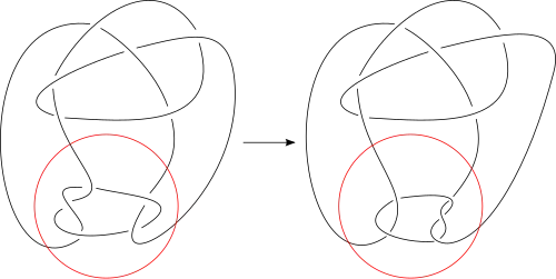
    The prime Kinoshita–Terasaka knot (11n42) and the prime Conway knot (11n34) respectively, and how they are related by mutation.

    In the mathematical field of knot theory, a mutation is an operation on a knot that can produce different knots. Suppose K is a knot given in the form of a knot diagram. Consider a disc D in the projection plane of the diagram whose boundary circle intersects K exactly four times. We may suppose that (after planar isotopy) the disc is geometrically round and the four points of intersection on its boundary with K are equally spaced. The part of the knot inside the disc is a tangle. There are two reflections that switch pairs of endpoints of the tangle. There is also a rotation that results from composition of the reflections. A mutation replaces the original tangle by a tangle given by any of these operations. The result will always be a knot and is called a mutant of K.

    Mutants can be difficult to distinguish as they have a number of the same invariants. They have the same hyperbolic volume (by a result of Ruberman), and have the same HOMFLY polynomials.

    Examples

    • Conway and Kinoshita-Terasaka mutant pair, distinguished as knot genus 3 and 2, respectively.

    References

    Further reading

    • Colin Adams, The Knot Book, American Mathematical Society, ISBN 0-8050-7380-9

    External links


    This article is adapted from “Mutation (knot theory)” on Wikipedia, written by its contributors, and used under CC BY-SA 4.0. Text on this page is available under the same licence. Source snapshot: Wikipedia via Kiwix, 2026-07-20.

  • Alternating knot

    Alternating knot
    One of three non-alternating knots with crossing number 8

    In knot theory, a knot or link diagram is alternating if the crossings alternate under, over, under, over, as one travels along each component of the link. A link is alternating if it has an alternating diagram.

    Many of the knots with crossing number less than 10 are alternating. This fact and useful properties of alternating knots, such as the Tait conjectures, was what enabled early knot tabulators, such as Tait, to construct tables with relatively few mistakes or omissions. The simplest non-alternating prime knots have 8 crossings (and there are three such: 819, 820, 821).

    It is conjectured that as the crossing number increases, the percentage of knots that are alternating goes to 0 exponentially quickly.

    Alternating links end up having an important role in knot theory and 3-manifold theory, due to their complements having useful and interesting geometric and topological properties. This led Ralph Fox to ask, “What is an alternating knot?” By this he was asking what non-diagrammatic properties of the knot complement would characterize alternating knots.[1]

    In November 2015, Joshua Evan Greene published a preprint that established a characterization of alternating links in terms of definite spanning surfaces, i.e. a definition of alternating links (of which alternating knots are a special case) without using the concept of a link diagram.[2]

    Various geometric and topological information is revealed in an alternating diagram. Primeness and splittability of a link is easily seen from the diagram. The crossing number of a reduced, alternating diagram is the crossing number of the knot. This last is one of the celebrated Tait conjectures.

    An alternating knot diagram is in one-to-one correspondence with a planar graph. Each crossing is associated with an edge and half of the connected components of the complement of the diagram are associated with vertices in a checker board manner.

    Alternating knot

    Alternating knot

    Tait conjectures

    The Tait conjectures are:

    1. Any reduced diagram of an alternating link has the fewest possible crossings.
    2. Any two reduced diagrams of the same alternating knot have the same writhe.
    3. Given any two reduced alternating diagrams D1 and D2 of an oriented, prime alternating link: D1 may be transformed to D2 by means of a sequence of certain simple moves called flypes. Also known as the Tait flyping conjecture.[3]

    Morwen Thistlethwaite, Louis Kauffman and K. Murasugi proved the first two Tait conjectures in 1987 and Morwen Thistlethwaite and William Menasco proved the Tait flyping conjecture in 1991.

    Hyperbolic volume

    Menasco, applying Thurston’s hyperbolization theorem for Haken manifolds, showed that any prime, non-split alternating link is hyperbolic, i.e. the link complement has a hyperbolic geometry, unless the link is a torus link.

    Thus hyperbolic volume is an invariant of many alternating links. Marc Lackenby has shown that the volume has upper and lower linear bounds as functions of the number of twist regions of a reduced, alternating diagram.

    References

    1. Lickorish, W. B. Raymond (1997), “Geometry of Alternating Links”, An Introduction to Knot Theory, Graduate Texts in Mathematics, vol. 175, Springer-Verlag, New York, pp. 32–40, doi:10.1007/978-1-4612-0691-0_4, ISBN 0-387-98254-X, MR 1472978; see in particular p. 32
    2. Greene, Joshua (2017). “Alternating links and definite surfaces”. Duke Mathematical Journal. 166 (11). arXiv:1511.06329. doi:10.1215/00127094-2017-0004. S2CID 59023367.
    3. Weisstein, Eric W. “Tait’s Knot Conjectures”. MathWorld. Accessed: May 5, 2013.

    Further reading

    External links


    This article is adapted from “Alternating knot” on Wikipedia, written by its contributors, and used under CC BY-SA 4.0. Text on this page is available under the same licence. Source snapshot: Wikipedia via Kiwix, 2026-07-20.

  • Murasugi sum

    In knot theory, a Murasugi sum is a way of combining the Seifert surfaces of two knots or links, given with embeddings in space of each knot and of a Seifert surface for each knot, to produce another Seifert surface of another knot or link. It was introduced by Kunio Murasugi, who used it to compute the genus[1] and Alexander polynomials[2] of certain alternating knots. When the two given Seifert surfaces have the minimum genus for their knot, the same is true for their Murasugi sum.[3] However, the genus of non-minimal-genus Seifert surfaces does not behave as predictably under Murasugi sums.[4]

    References

    1. Murasugi, Kunio (1958), “On the genus of the alternating knot. I, II”, Journal of the Mathematical Society of Japan, 10: 94–105, 235–248, doi:10.2969/jmsj/01010094, MR 0099664
    2. Murasugi, Kunio (1963), “On a certain subgroup of the group of an alternating link”, American Journal of Mathematics, 85: 544–550, doi:10.2307/2373107, MR 0157375
    3. Gabai, David (1983), “The Murasugi sum is a natural geometric operation”, Low-dimensional topology (San Francisco, Calif., 1981), Contemporary Mathematics, vol. 20, American Mathematical Society, pp. 131–143, doi:10.1090/conm/020/718138, ISBN 0-8218-5016-4, MR 0718138
    4. Thompson, Abigail (1994), “A note on Murasugi sums”, Pacific Journal of Mathematics, 163 (2): 393–395, MR 1262303


    This article is adapted from “Murasugi sum” on Wikipedia, written by its contributors, and used under CC BY-SA 4.0. Text on this page is available under the same licence. Source snapshot: Wikipedia via Kiwix, 2026-07-20.

  • Algebraic link

    Algebraic link
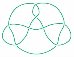
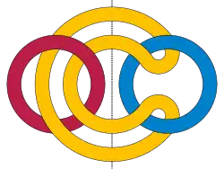
    Decomposition of the Borromean rings by a Conway sphere (black dotted vertical midline) into two 2-tangles, showing that the Borromean rings form an algebraic link

    In the mathematical field of knot theory, an algebraic link is a link that can be decomposed by Conway spheres into 2-tangles.[1] Algebraic links are also called arborescent links.[2]
    Although algebraic links and algebraic tangles were originally defined by John H. Conway as having two pairs of open ends, they were subsequently generalized to more pairs.[3]

    References

    1. Thistlethwaite, Morwen B. (1991). “On the algebraic part of an alternating link”. Pacific Journal of Mathematics. 151 (2): 317–333. MR 1132393.
    2. Gabai, David (1986). “Genera of the arborescent links”. Memoirs of the American Mathematical Society. 59 (339): 1–98. doi:10.1090/memo/0339.
    3. Hazewinkel, Michiel (2001). Encyclopaedia of Mathematics, Supplement III, Volume 13. Springer. p. 34. ISBN 9781556080104..

    This article is adapted from “Algebraic link” on Wikipedia, written by its contributors, and used under CC BY-SA 4.0. Text on this page is available under the same licence. Source snapshot: Wikipedia via Kiwix, 2026-07-20.

  • Munter hitch

    Munter hitch
    Munter hitch
    Names Munter hitch, HMS, Italian hitch, Flip-Flop knot, and the first part of the knot is formed in the same manner as the Crossing hitch (ABoK #1818, #1725, #1797)
    Category Hitch
    Related Half hitch, Zigzag Knot (ABoK #1195), Monster Munter
    Releasing Non-jamming
    Typical use Belaying
    Caveat Wears out the rope when used for descending

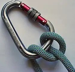
    The Munter hitch, also known as the Italian hitch, mezzo barcaiolo is a simple adjustable knot, commonly used by climbers, cavers, and rescuers to control friction in a life-lining or belay system. It is often mistakenly identified as the crossing hitch,[1] however in the cross hitch the line does not return along its original path. To climbers, this hitch is also known as HMS, the abbreviation for the German term Halbmastwurfsicherung, meaning half clove hitch belay. This technique can be used with a special “pear-shaped” HMS locking carabiner, or any locking carabiner wide enough to take two turns of the rope.

    In the late 1950s, three Italian climbers, Mario Bisaccia, Franco Garda and Pietro Gilardoni developed a new belay technique called the “Mezzo Barcaiolo” (MB) meaning; “a half of the knot, which is used by the sailors to secure a boat to a bollard in a harbor.”[2] The “MB” came to be known as the Munter hitch after Werner Munter, a Swiss mountain guide popularized its use in mountaineering in the 1970s.[3] This hitch was studied and then promoted for its use in the mountains (being officially recognized by the UIAA towards the end of the sixties), by the Italian Alpine Club and, in particular, by its Central Commission for Materials and Techniques.[4]

    The hitch is simply a set of wraps using a rope or cord around an object, generally a round object like a pipe, pole or more commonly, a carabiner. Its main use is as a friction device for controlling the rate of descent in belay systems.

    Method of operation

    The Munter hitch creates friction by having the rope rub on itself and on the object it has been wrapped around. There is no localized abrasion on any part of the rope as it is a continuously moving hitch. One very useful aspect of the Munter is its reversibility; it can be pulled from either side of the rope and it still works just as effectively. The Munter hitch is a self regulating hitch. The heavier the load the tighter the bends in the hitch become and therefore creating more friction and self regulating.

    Use for rappeling

    Munter hitch
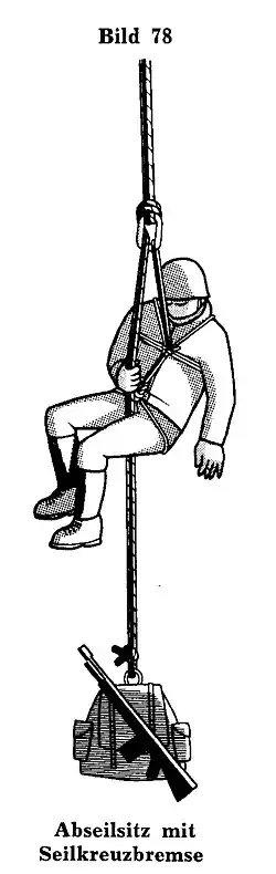
    A soldier abseiling with a Munter hitch, depicted in a German military publication from 1966.

    This hitch can be used to rappel or abseil down a vertical or semi-vertical wall, although it is not recommended as it causes severe twisting of the rope. Proper training should be undertaken before using the Munter hitch to rappel. Using this method to rappel is very hard on rope because of the rope on rope contact and is generally considered an emergency option only.

    Use as load releasable tie off

    As with most belay devices and some hitches the Munter can be tied off to maintain tension in a manner which is easily released under tension, often referred to as a Munter-Mule-Overhand or MMO.

    The control rope (the rope not going to the load) is tied to the load rope with a mule knot (aka halter hitch)  not a noose (slipped overhand)  and the bight (loop) that sticks out is tied in an overhand around the load rope. A carabiner is then sometimes clipped through the end of the bight and around the load rope.

    Examples of when a tie off would be employed include:

    • tensioning the line for use as a track line
    • fall restraint line
    • restraining/guying purposes.

    When a belayer needs to transfer the load from their harness to the anchor to escape the system:
    a rope grab (mechanical or friction knot/Prusik) is placed on the load line towards the load, rope is terminated on the rope grab (or the tails of accessory cord are used when using a cordelette with a Prusik as a rope grab) and runs back to the anchor where a Munter mule is tied under tension. The load can then be lowered (transferred) from the original belay onto the Munter Mule via the rope grab. The new line is often consider independent of the safety system so the original belay needs to be maintained throughout the process and secured back to the anchor before the system can be left unattended.

    Use as a belay

    A belay system incorporating the Munter hitch is the same as any other belay system, which incorporates a belayer to tend the rope and an anchor, which secures the belay system and belayer.

    There are several advantages to the Munter hitch. It requires no additional hardware other than a carabiner. It is also the most common belay system which locks with the brake hand in line with the load, and as such is a more suitable method for direct belays than using a normal belay plate.[5] This can be useful when the anchor, carabiner and Munter hitch are above or behind the belayer whilst attention is paid to the loaded end of the rope. It can also more effectively dissipate heat than a belay device because no two surfaces of the rope are in contact with each other for more than an instant.

    However, it places more bends in a rope than other belay methods, and creates significantly more friction on the outer sheath. Another disadvantage is that it can introduce significant twists to the rope. It is a versatile knot to know and can be used for full rope length vertical descents without the need for gloves.

    The friction of the rope against the screw on the carabiner can cause the screw to undo and the carabiner to open, potentially weakening the strength of the carabiner, or allowing the rope to escape the carabiner completely. Therefore the hitch has to be tied correctly with the braking end on the opposite side of the carabiner than the gate is.

    Military use

    The Munter hitch is taught on Australian military roping courses as a simple and effective method for descending steep or overhanging terrain with combat equipment and can also be used for lowering heavy stores or casualties, the only equipment required being a harness or webbing seat, a locking carabiner, and a rope.

    Arboreal usage

    For the recreational tree climber or working arborist, the Munter is useful to know as a reliable lowering knot for moderate loads. This hitch performs well on both 16 strand arborist climbing lines and the 11 mm double braid lines.

    Tower technicians

    Tower technicians also use this knot for lowering loads, and tagging heavy loads while hoisting. It is commonly referred to in the tower industry as a tag knot.

    See also

    References

    1. Clifford W. Ashley. The Ashley Book of Knots. Doubleday, 1944. p. 306.
    2. Phillips, Ken. “NPS Technical Rescue Handbook” (PDF). Mountain Rescue Association. National Park Service. Retrieved 4 March 2021.
    3. George, Caroline. “Munter Magic”. Climbing Magazine. Retrieved 2019-04-14.
    4. “Cai Materiali”. CAI Materiali. Retrieved 4 March 2021.
    5. S. Long, The Climbing Handbook, 64

    External links


    This article is adapted from “Munter hitch” on Wikipedia, written by its contributors, and used under CC BY-SA 4.0. Text on this page is available under the same licence. Source snapshot: Wikipedia via Kiwix, 2026-07-20.

  • Alexander polynomial

    In mathematics, the Alexander polynomial is a knot invariant which assigns a polynomial with integer coefficients to each knot type. James Waddell Alexander II discovered this, the first knot polynomial, in 1923. In 1969, John Conway showed a version of this polynomial, now called the Alexander–Conway polynomial, could be computed using a skein relation, although its significance was not realized until the discovery of the Jones polynomial in 1984. Soon after Conway’s reworking of the Alexander polynomial, it was realized that a similar skein relation was exhibited in Alexander’s paper on his polynomial.[a]

    Definition

    Let K be a knot in the 3-sphere. Let X be the infinite cyclic cover of the knot complement of K. This covering can be obtained by cutting the knot complement along a Seifert surface of K and gluing together infinitely many copies of the resulting manifold with boundary in a cyclic manner. There is a covering transformation t acting on X. Consider the first homology (with integer coefficients) of X, denoted H 1 ( X ) {\displaystyle H_{1}(X)} {\displaystyle H_{1}(X)}. The transformation t acts on the homology and so we can consider H 1 ( X ) {\displaystyle H_{1}(X)} {\displaystyle H_{1}(X)} a module over the ring of Laurent polynomials Z [ t , t 1 ] {\displaystyle \mathbb {Z} [t,t^{-1}]} {\displaystyle \mathbb {Z} [t,t^{-1}]}. This is called the Alexander invariant or Alexander module.

    The module is finitely presentable; a presentation matrix for this module is called the Alexander matrix. If the number of generators, r {\displaystyle r} {\displaystyle r}, is less than or equal to the number of relations, s {\displaystyle s} {\displaystyle s} , then we consider the ideal generated by all r × r {\displaystyle r\times r} {\displaystyle r\times r} minors of the matrix; this is the zeroth Fitting ideal or Alexander ideal and does not depend on choice of presentation matrix. If r > s {\displaystyle r>s} {\displaystyle r>s}, set the ideal equal to 0. If the Alexander ideal is principal, take a generator; this is called an Alexander polynomial of the knot. Since this is only unique up to multiplication by the Laurent monomial ± t n {\displaystyle \pm t^{n}} {\displaystyle \pm t^{n}}, one often fixes a particular unique form. Alexander’s choice of normalization is to make the polynomial have a positive constant term.

    Alexander proved that the Alexander ideal is nonzero and always principal. Thus an Alexander polynomial always exists, and is clearly a knot invariant, denoted Δ K ( t ) {\displaystyle \Delta _{K}(t)} {\displaystyle \Delta _{K}(t)}. It turns out that the Alexander polynomial of a knot is the same polynomial for the mirror image knot. In other words, it cannot distinguish between a knot and its mirror image.

    Computing the polynomial

    The following procedure for computing the Alexander polynomial was given by J. W. Alexander in his paper.[2]

    Take an oriented diagram of the knot with n {\displaystyle n} {\displaystyle n} crossings; there are n + 2 {\displaystyle n+2} {\displaystyle n+2} regions of the knot diagram. To work out the Alexander polynomial, first one must create an incidence matrix of size ( n , n + 2 ) {\displaystyle (n,n+2)} {\displaystyle (n,n+2)}. The n {\displaystyle n} {\displaystyle n} rows correspond to the n {\displaystyle n} {\displaystyle n} crossings, and the n + 2 {\displaystyle n+2} {\displaystyle n+2} columns to the regions. The values for the matrix entries are either 0 , 1 , 1 , t , t {\displaystyle 0,1,-1,t,-t} {\displaystyle 0,1,-1,t,-t}.

    Consider the entry corresponding to a particular region and crossing. If the region is not adjacent to the crossing, the entry is 0. If the region is adjacent to the crossing, the entry depends on its location. The following table gives the entry, determined by the location of the region at the crossing from the perspective of the incoming undercrossing line.

    on the left before undercrossing: t {\displaystyle -t} {\displaystyle -t}
    on the right before undercrossing: 1 {\displaystyle 1} {\displaystyle 1}
    on the left after undercrossing: t {\displaystyle t} {\displaystyle t}
    on the right after undercrossing: 1 {\displaystyle -1} {\displaystyle -1}

    Remove two columns corresponding to adjacent regions from the matrix, and work out the determinant of the new n × n {\displaystyle n\times n} {\displaystyle n\times n} matrix. Depending on the columns removed, the answer will differ by multiplication by ± t n {\displaystyle \pm t^{n}} {\displaystyle \pm t^{n}}, where the power of n {\displaystyle n} {\displaystyle n} is not necessarily the number of crossings in the knot. To resolve this ambiguity, divide out the largest possible power of t {\displaystyle t} {\displaystyle t} and multiply by 1 {\displaystyle -1} {\displaystyle -1} if necessary, so that the constant term is positive. This gives the Alexander polynomial. For example, this shows immediately that the Alexander polynomial of the unknot is 1 (though this follows also immediately from the definition).

    The Alexander polynomial can also be computed from the Seifert matrix.

    After the work of J. W. Alexander, Ralph Fox considered a copresentation of the knot group π 1 ( S 3 K ) {\displaystyle \pi _{1}(S^{3}\backslash K)} {\displaystyle \pi _{1}(S^{3}\backslash K)}, and introduced non-commutative differential calculus, which also permits one to compute Δ K ( t ) {\displaystyle \Delta _{K}(t)} {\displaystyle \Delta _{K}(t)}.[3][b]

    Basic properties of the polynomial

    The Alexander polynomial is symmetric: Δ K ( t 1 ) = Δ K ( t ) {\displaystyle \Delta _{K}(t^{-1})=\Delta _{K}(t)} {\displaystyle \Delta _{K}(t^{-1})=\Delta _{K}(t)} for all knots K.

    From the point of view of the definition, this is an expression of the Poincaré Duality isomorphism H 1 X ¯ H o m Z [ t , t 1 ] ( H 1 X , G ) {\displaystyle {\overline {H_{1}X}}\simeq \mathrm {Hom} _{\mathbb {Z} [t,t^{-1}]}(H_{1}X,G)} {\displaystyle {\overline {H_{1}X}}\simeq \mathrm {Hom} _{\mathbb {Z} [t,t^{-1}]}(H_{1}X,G)} where G {\displaystyle G} {\displaystyle G} is the quotient of the field of fractions of Z [ t , t 1 ] {\displaystyle \mathbb {Z} [t,t^{-1}]} {\displaystyle \mathbb {Z} [t,t^{-1}]} by Z [ t , t 1 ] {\displaystyle \mathbb {Z} [t,t^{-1}]} {\displaystyle \mathbb {Z} [t,t^{-1}]}, considered as a Z [ t , t 1 ] {\displaystyle \mathbb {Z} [t,t^{-1}]} {\displaystyle \mathbb {Z} [t,t^{-1}]}-module, and where H 1 X ¯ {\displaystyle {\overline {H_{1}X}}} {\displaystyle {\overline {H_{1}X}}} is the conjugate Z [ t , t 1 ] {\displaystyle \mathbb {Z} [t,t^{-1}]} {\displaystyle \mathbb {Z} [t,t^{-1}]}-module to H 1 X {\displaystyle H_{1}X} {\displaystyle H_{1}X} ie: as an abelian group it is identical to H 1 X {\displaystyle H_{1}X} {\displaystyle H_{1}X} but the covering transformation t {\displaystyle t} {\displaystyle t} acts by t 1 {\displaystyle t^{-1}} {\displaystyle t^{-1}}.

    Furthermore, the Alexander polynomial evaluates to a unit on 1: Δ K ( 1 ) = ± 1 {\displaystyle \Delta _{K}(1)=\pm 1} {\displaystyle \Delta _{K}(1)=\pm 1}.
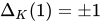
    From the point of view of the definition, this is an expression of the fact that the knot complement is a homology circle, generated by the covering transformation t {\displaystyle t} {\displaystyle t}. More generally if M {\displaystyle M} {\displaystyle M} is a 3-manifold such that r a n k ( H 1 M ) = 1 {\displaystyle rank(H_{1}M)=1} {\displaystyle rank(H_{1}M)=1} it has an Alexander polynomial Δ M ( t ) {\displaystyle \Delta _{M}(t)} {\displaystyle \Delta _{M}(t)} defined as the order ideal of its infinite-cyclic covering space. In this case Δ M ( 1 ) {\displaystyle \Delta _{M}(1)} {\displaystyle \Delta _{M}(1)} is, up to sign, equal to the order of the torsion subgroup of H 1 M {\displaystyle H_{1}M} {\displaystyle H_{1}M}.

    The value of the Alexander polynomial evaluated at -1 is known as the determinant of the knot. Every integral Laurent polynomial which is both symmetric and evaluates to a unit at 1 is the Alexander polynomial of a knot.[4]

    Geometric significance of the polynomial

    Since the Alexander ideal is principal, Δ K ( t ) = 1 {\displaystyle \Delta _{K}(t)=1} {\displaystyle \Delta _{K}(t)=1} if and only if the commutator subgroup of the knot group is perfect (i.e. equal to its own commutator subgroup).

    For a topologically slice knot, the Alexander polynomial satisfies the Fox–Milnor condition Δ K ( t ) = f ( t ) f ( t 1 ) {\displaystyle \Delta _{K}(t)=f(t)f(t^{-1})} {\displaystyle \Delta _{K}(t)=f(t)f(t^{-1})} where f ( t ) {\displaystyle f(t)} {\displaystyle f(t)} is some other integral Laurent polynomial.

    Twice the knot genus is bounded below by the degree of the Alexander polynomial.

    Michael Freedman proved that a knot in the 3-sphere is topologically slice; i.e., bounds a “locally-flat” topological disc in the 4-ball, if the Alexander polynomial of the knot is trivial.[5]

    Kauffman describes the first construction of the Alexander polynomial via state sums derived from physical models. A survey of these topics and other connections with physics are given in.[6][7]

    There are other relations with surfaces and smooth 4-dimensional topology. For example, under certain assumptions, there is a way of modifying a smooth 4-manifold by performing a surgery that consists of removing a neighborhood of a two-dimensional torus and replacing it with a knot complement crossed with S1. The result is a smooth 4-manifold homeomorphic to the original, though now the Seiberg–Witten invariant has been modified by multiplication with the Alexander polynomial of the knot.[8]

    Knots with symmetries are known to have restricted Alexander polynomials.[9] Nonetheless, the Alexander polynomial can fail to detect some symmetries, such as strong invertibility.

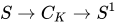
    If the knot complement fibers over the circle, then the Alexander polynomial of the knot is known to be monic (the coefficients of the highest and lowest order terms are equal to ± 1 {\displaystyle \pm 1} {\displaystyle \pm 1}). In fact, if S C K S 1 {\displaystyle S\to C_{K}\to S^{1}} {\displaystyle S\to C_{K}\to S^{1}} is a fiber bundle where C K {\displaystyle C_{K}} {\displaystyle C_{K}} is the knot complement, let g : S S {\displaystyle g:S\to S} {\displaystyle g:S\to S} represent the monodromy, then Δ K ( t ) = D e t ( t I g ) {\displaystyle \Delta _{K}(t)={\rm {Det}}(tI-g_{*})} {\displaystyle \Delta _{K}(t)={\rm {Det}}(tI-g_{*})} where g : H 1 S H 1 S {\displaystyle g_{*}\colon H_{1}S\to H_{1}S} {\displaystyle g_{*}\colon H_{1}S\to H_{1}S} is the induced map on homology.

    Relations to satellite operations

    If a knot K {\displaystyle K} {\displaystyle K} is a satellite knot with pattern knot K {\displaystyle K’} {\displaystyle K'} (there exists an embedding f : S 1 × D 2 S 3 {\displaystyle f:S^{1}\times D^{2}\to S^{3}} {\displaystyle f:S^{1}\times D^{2}\to S^{3}} such that K = f ( K ) {\displaystyle K=f(K’)} {\displaystyle K=f(K')}, where S 1 × D 2 S 3 {\displaystyle S^{1}\times D^{2}\subset S^{3}} {\displaystyle S^{1}\times D^{2}\subset S^{3}} is an unknotted solid torus containing K {\displaystyle K’} {\displaystyle K'}), then Δ K ( t ) = Δ f ( S 1 × { 0 } ) ( t a ) Δ K ( t ) {\displaystyle \Delta _{K}(t)=\Delta _{f(S^{1}\times \{0\})}(t^{a})\Delta _{K’}(t)} {\displaystyle \Delta _{K}(t)=\Delta _{f(S^{1}\times \{0\})}(t^{a})\Delta _{K'}(t)}, where a Z {\displaystyle a\in \mathbb {Z} } {\displaystyle a\in \mathbb {Z} } is the integer that represents K S 1 × D 2 {\displaystyle K’\subset S^{1}\times D^{2}} {\displaystyle K'\subset S^{1}\times D^{2}} in H 1 ( S 1 × D 2 ) = Z {\displaystyle H_{1}(S^{1}\times D^{2})=\mathbb {Z} } {\displaystyle H_{1}(S^{1}\times D^{2})=\mathbb {Z} }.

    Examples: For a connect-sum Δ K 1 # K 2 ( t ) = Δ K 1 ( t ) Δ K 2 ( t ) {\displaystyle \Delta _{K_{1}\#K_{2}}(t)=\Delta _{K_{1}}(t)\Delta _{K_{2}}(t)} {\displaystyle \Delta _{K_{1}\#K_{2}}(t)=\Delta _{K_{1}}(t)\Delta _{K_{2}}(t)}. If K {\displaystyle K} {\displaystyle K} is an untwisted Whitehead double, then Δ K ( t ) = ± 1 {\displaystyle \Delta _{K}(t)=\pm 1} {\displaystyle \Delta _{K}(t)=\pm 1}.

    Knots with the same Alexander polynomial

    The Alexander polynomial is not a complete invariant for knots, that is two distinct knots may have the same Alexander polynomial. For example, according to the database KnotInfo[10] there occurs only 212 unique Alexander polynomials among the 250 knots with up to 10 crossings.

    The Alexander polynomial does not detect the unknot: there are infinitely many knots which have Alexander polynomial equal to 1. For example, these include every Whitehead double of an untwisted knot. Explicit examples of knots with few crossings having Alexander polynomial 1 are the Conway knot and the Kinoshita–Terasaka knot, both with 11 crossings. In contrast, it is still unknown whether the Jones polynomial (or the stronger HOMFLY polynomial) determines the unknot.

    The Alexander polynomial does not detect primeness of a knot, that is, a prime knot may have the same Alexander polynomial as a composite knot. There are many more properties which are not detected by the Alexander polynomial.[11]

    Alexander–Conway polynomial

    Alexander proved the Alexander polynomial satisfies a skein relation. John Conway later rediscovered this in a different form and showed that the skein relation together with a choice of value on the unknot was enough to determine the polynomial. Conway’s version is a polynomial in z with integer coefficients, denoted ( z ) {\displaystyle \nabla (z)} {\displaystyle \nabla (z)} and called the Alexander–Conway polynomial (also known as Conway polynomial or Conway–Alexander polynomial).

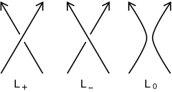
    Suppose we are given an oriented link diagram, where L + , L , L 0 {\displaystyle L_{+},L_{-},L_{0}} {\displaystyle L_{+},L_{-},L_{0}} are link diagrams resulting from crossing and smoothing changes on a local region of a specified crossing of the diagram, as indicated in the figure.

    Alexander polynomial

    Here are Conway’s skein relations:

    • ( O ) = 1 {\displaystyle \nabla (O)=1} {\displaystyle \nabla (O)=1} (where O is any diagram of the unknot)
    • ( L + ) ( L ) = z ( L 0 ) {\displaystyle \nabla (L_{+})-\nabla (L_{-})=z\nabla (L_{0})} {\displaystyle \nabla (L_{+})-\nabla (L_{-})=z\nabla (L_{0})}

    The relationship to the standard Alexander polynomial is given by Δ L ( t 2 ) = L ( t t 1 ) {\displaystyle \Delta _{L}(t^{2})=\nabla _{L}(t-t^{-1})} {\displaystyle \Delta _{L}(t^{2})=\nabla _{L}(t-t^{-1})}. Here Δ L {\displaystyle \Delta _{L}} {\displaystyle \Delta _{L}} must be properly normalized (by multiplication of ± t n / 2 {\displaystyle \pm t^{n/2}} {\displaystyle \pm t^{n/2}}) to satisfy the skein relation Δ ( L + ) Δ ( L ) = ( t 1 / 2 t 1 / 2 ) Δ ( L 0 ) {\displaystyle \Delta (L_{+})-\Delta (L_{-})=(t^{1/2}-t^{-1/2})\Delta (L_{0})} {\displaystyle \Delta (L_{+})-\Delta (L_{-})=(t^{1/2}-t^{-1/2})\Delta (L_{0})}. Note that this relation gives a Laurent polynomial in t1/2.

    See knot theory for an example computing the Conway polynomial of the trefoil.

    Relation to Floer homology

    Using pseudo-holomorphic curves, Ozsváth-Szabó[12] and Rasmussen[13] associated a bigraded abelian group, called knot Floer homology, to each isotopy class of knots. The graded Euler characteristic of knot Floer homology is the Alexander polynomial. While the Alexander polynomial gives a lower bound on the genus of a knot, Ozsváth-Szabó[14] showed that knot Floer homology detects the genus. Similarly, while the Alexander polynomial gives an obstruction to a knot complement fibering over the circle, Ni[15] showed that knot Floer homology completely determines when a knot complement fibers over the circle. The knot Floer homology groups are part of the Heegaard Floer homology family of invariants; see Floer homology for further discussion.

    Notes

    1. Alexander describes his skein relation toward the end of his paper under the heading “miscellaneous theorems”, which is possibly why it got lost. Joan Birman mentions in her paper that Mark Kidwell brought her attention to Alexander’s relation in 1970.[1]
    2. Detailed exposition of this approach about higher Alexander polynomials can be found in Crowell & Fox (1963).

    References

    1. Birman 1993.
    2. Alexander 1928.
    3. Fox 1961.
    4. Kawauchi 2012, Theorem 11.5.3, p. 150. Kawauchi credits this result to Kondo, H. (1979), “Knots of unknotting number 1 and their Alexander polynomials”, Osaka J. Math. 16: 551-559, and to Sakai, T. (1977), “A remark on the Alexander polynomials of knots”, Math. Sem. Notes Kobe Univ. 5: 451~456.
    5. Freedman & Quinn 1990.
    6. Kauffman 1983.
    7. Kauffman 2012.
    8. Fintushel & Stern 1998.
    9. Kawauchi 2012, symmetry section.
    10. “KnotInfo”. KnotInfo. Retrieved 2025-09-17.
    11. Cromwell, P. R. (1991). “Some infinite families of satellite knots with given Alexander polynomial”. Mathematika. 38 (1). Wiley: 156–169. doi:10.1112/s0025579300006513. ISSN 0025-5793.
    12. Ozsváth & Szabó 2004.
    13. Rasmussen 2003.
    14. Ozsváth & Szabó 2004b.
    15. Ni 2007.

    Sources

    • Adams, Colin C. (2004) [1994]. The Knot Book: An elementary introduction to the mathematical theory of knots. American Mathematical Society. ISBN 978-0-8218-3678-1. (accessible introduction utilizing a skein relation approach)
    • Alexander, J. W. (1928). “Topological Invariants of Knots and Links” (PDF). Transactions of the American Mathematical Society. 30 (2): 275–306. doi:10.1090/S0002-9947-1928-1501429-1. JSTOR 1989123.
    • Birman, Joan (1993). “New points of view in knot theory”. Bull. Amer. Math. Soc. N.S. 28 (2): 253–287. arXiv:math/9304209. doi:10.1090/S0273-0979-1993-00389-6.
    • Crowell, Richard; Fox, Ralph (1963). Introduction to Knot Theory. Ginn and Co. after 1977 Springer Verlag.
    • Fintushel, Ronald; Stern, Ronald J. (October 1998). “Knots, links, and 4-manifolds”. Inventiones Mathematicae. 134 (2): 363–400. arXiv:dg-ga/9612014. Bibcode:1998InMat.134..363F. doi:10.1007/s002220050268. ISSN 0020-9910. MR 1650308. S2CID 3752148.
    • Fox, Ralph (1961). “A quick trip through knot theory”. In Fort, M.K. (ed.). Proceedings of the University of Georgia Topology Institute. Englewood Cliffs. N. J.: Prentice-Hall. pp. 120–167. OCLC 73203715.
    • Freedman, Michael H.; Quinn, Frank (1990). Topology of 4-manifolds. Princeton Mathematical Series. Vol. 39. Princeton University Press. ISBN 978-0-691-08577-7.
    • Kauffman, Louis (2006) [1983]. Formal Knot Theory. Courier. ISBN 978-0-486-45052-0.
    • Kauffman, Louis (2012). Knots and Physics (4th ed.). World Scientific Publishing Company. ISBN 978-981-4383-00-4.
    • Kawauchi, Akio (2012) [1996]. A Survey of Knot Theory. Birkhäuser. ISBN 978-3-0348-9227-8. (covers several different approaches, explains relations between different versions of the Alexander polynomial)
    • Ni, Yi (2007). “Knot Floer homology detects fibred knots”. Inventiones Mathematicae. Invent. Math. 170 (3): 577–608. arXiv:math/0607156. Bibcode:2007InMat.170..577N. doi:10.1007/s00222-007-0075-9. S2CID 119159648.
    • Ozsváth, Peter; Szabó, Zoltán (2004). “Holomorphic disks and knot invariants”. Advances in Mathematics. 186 (1): 58–116. arXiv:math/0209056. Bibcode:2002math……9056O. doi:10.1016/j.aim.2003.05.001. S2CID 11246611.
    • Ozsváth, Peter; Szabó, Zoltán (2004b). “Holomorphic disks and genus bounds”. Geometry and Topology. 8 (2004): 311–334. arXiv:math/0311496. doi:10.2140/gt.2004.8.311. S2CID 11374897.
    • Rasmussen, Jacob (2003). Floer homology and knot complements (Thesis). Harvard University. p. 6378. arXiv:math/0306378. Bibcode:2003math……6378R.
    • Rolfsen, Dale (1990). Knots and Links (2nd ed.). Publish or Perish. ISBN 978-0-914098-16-4. (explains classical approach using the Alexander invariant; knot and link table with Alexander polynomials)

    External links


    This article is adapted from “Alexander polynomial” on Wikipedia, written by its contributors, and used under CC BY-SA 4.0. Text on this page is available under the same licence. Source snapshot: Wikipedia via Kiwix, 2026-07-20.
  • Mooring hitch

    Mooring hitch
    Mooring hitch
    Category Hitch
    Origin Ancient
    Related Lapp knot
    Releasing Non-jamming
    Typical use tie a boat to a post, quick-release

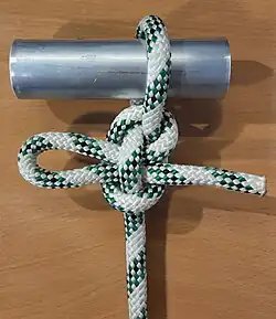
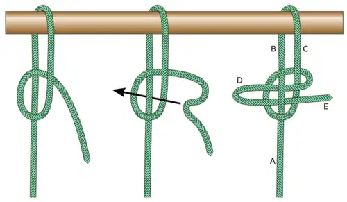
    The mooring hitch can be used to tie a small boat to a post, pole, bollard or similar. As it is a quick-release knot, it can be easily untied by pulling the working end E.[1] If the working end is long enough, this can be done from the boat.[2] It is considered rather insecure though.[2][3]

    Mooring hitch
    Tying the mooring hitch

    The mooring hitch can slide along the standing part (A-B); a pull on the other parts (C,D) can lock it into place, forming a fixed loop also known as the Lapp knot.

    Name

    The name mooring hitch sometimes refers to other knots like the Tugboat hitch.

    Alternatives

    • The slipped buntline hitch is a probably more secure quick-release hitch.
    • The tumble hitch is also a quick-release hitch, and it becomes completely undone and separated from the post it was tied to (exploding knot).

    References

    1. Budworth, Geoffrey (1997). The Complete Book of Knots. The Lyons Press. p. 46. ISBN 1-55821-632-4.
    2. 1 2 Holtzman, Bob (2015). The Field Guide to Knots. Quid Publishing, LLC. p. 158. ISBN 978-1-61519-276-2.
    3. “Mooring Hitch”. Animated Knots. Retrieved 2021-10-26.

    This article is adapted from “Mooring hitch” on Wikipedia, written by its contributors, and used under CC BY-SA 4.0. Text on this page is available under the same licence. Source snapshot: Wikipedia via Kiwix, 2026-07-20.
  • Alexander’s theorem

    Alexander's theorem
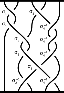
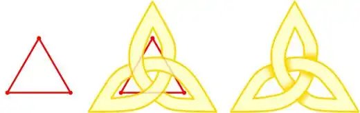
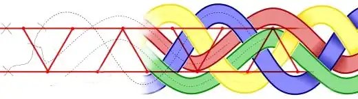
    This is a typical element of the braid group, which is used in the mathematical field of knot theory.

    In mathematics Alexander’s theorem states that every knot or link can be represented as a closed braid; that is, a braid in which the corresponding ends of the strings are connected in pairs. The theorem is named after James Waddell Alexander II, who published a proof in 1923.[1]

    Braids were first considered as a tool of knot theory by Alexander. His theorem gives a positive answer to the question Is it always possible to transform a given knot into a closed braid? A good construction example is found in Colin Adams’s book.[2]

    However, the correspondence between knots and braids is clearly not one-to-one: a knot may have many braid representations. For example, conjugate braids yield equivalent knots. This leads to a second fundamental question: Which closed braids represent the same knot type?
    This question is addressed in Markov’s theorem, which gives ‘moves’ relating any two closed braids that represent the same knot.

    References

    1. Alexander, James (1923). “A lemma on a system of knotted curves”. Proceedings of the National Academy of Sciences of the United States of America. 9 (3): 93–95. Bibcode:1923PNAS….9…93A. doi:10.1073/pnas.9.3.93. PMC 1085274. PMID 16576674.
    2. Adams, Colin C. (2004). The Knot Book. Revised reprint of the 1994 original. Providence, RI: American Mathematical Society. p. 130. ISBN 0-8218-3678-1. MR 2079925.


    This article is adapted from “Alexander's theorem” on Wikipedia, written by its contributors, and used under CC BY-SA 4.0. Text on this page is available under the same licence. Source snapshot: Wikipedia via Kiwix, 2026-07-20.
  • Monkey’s fist

    Monkey’s fist
    Monkey's fist
    Category Stopper
    Typical use tied at the end of a rope to serve as a weight or an anchor
    ABoK #2202
    Instructions

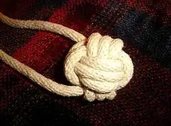
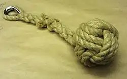
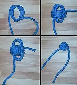
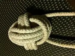
    A monkey’s fist or monkey paw is a type of knot, so named because it looks somewhat like a small bunched fist or paw. It is tied at the end of a rope to serve as a weight, making it easier to throw, and also as an ornamental knot. This type of weighted rope can be used as a hand-to-hand weapon, called a slungshot by sailors. It was also used in the past as an anchor in rock climbing, by stuffing it into a crack. It is still sometimes used today in sandstone, as in the Elbe Sandstone Mountains in Germany.

    Description

    Monkey's fist
    an ornamental monkey’s fist with a hard eye splice, custom-made at the chandlers Arthur Beale

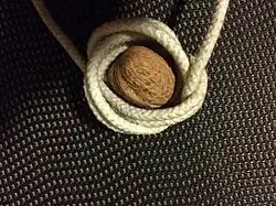
    The monkey’s fist is a spherical covering with six surface parts presenting a regular over-one-and-under-one weave. This weave is commonly doubled or tripled to present an appearance that superficially resembles a Turk’s-head. Like the Turk’s-head, the knot is tied with a single strand, but here the resemblance ceases. The Turk’s-head diagram consists of a single line; the common monkey’s fist diagram has three separate lines, which are best represented by three interlocking circles, in the best Ballantine tradition. To tie a knot on this diagram with a single strand, it is necessary to complete each circle in turn—that is, to double or triple it, as the case may be—and when this has been done to deflect the strand into another circle which is completed in turn before commencing the third and last circle.

    The monkey’s fist knot is most often used as the weight in a heaving line. The line would have the monkey’s fist on one end, an eye splice or bowline on the other, with about 30 feet (~10 metres) of line between. A lightweight feeder line would be tied to the bowline, then the weighted heaving line could be hurled between ship and dock. The other end of the lightweight line would be attached to a heavier-weight line, allowing it to be drawn to the target easily.

    The knot is often tied around a small weight, such as a stone, marble, tight fold of paper, grapeshot, or a piece of wood. However, this may be considered unsafe and therefore poor seamanship.
    The UK Maritime and Coastguard Agency’s (MCA) publication “Code of Safe Working Practices for Merchant Seamen”, Section 25.3.2, states that “heaving lines should be constructed with a ‘monkey’s fist’ at one end. To prevent personal injury, the ‘fist’ should be made only with rope and should not contain added weighting materials”.
    [2]

    Tying

    Monkey's fist
    tying the Monkeys fist

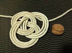
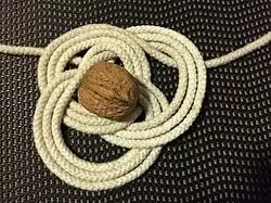
    The three coils of cordage in a monkey’s fist form in effect a set of Borromean rings in three dimensions. This is most obvious when tied flat. The rings should then be started near center, coiled from outside inwards, in all three set of rings, and the third set finished by letting the end exit through the triangular hole at the center. Subsequent tightening should let the outside edges curl to form an opposing triangular hole around the main part. This is suitable if a ring formed object is to be contained in the central cavity around the main part. If the object has no hole, it might be desirable to have the ends exit the knot at or near the central triangular hole.

    • Flat tying monkey’s fist knot
    • Step 1: tied flat
      Step 1: tied flat
    • Step 2: flat, with content in the middle
      Step 2: flat, with content in the middle
    • Step 3: loosely wrapping content
      Step 3: loosely wrapping content
    • Step 4: tightened around content
      Step 4: tightened around content

    Other applications

    Monkey's fist
    A cufflink made from a wire tied into a Monkey’s fist knot

    A monkey’s fist can be used on two ends of a tow lines of one side a fish net which is then thrown from one trawler to another, allowing the net to be cast and set between two boats so the trawl can be used between the two, in pair trawling[3] where the tow or catch is negotiated between both parties. This makes it easier to catch fish given the greater surface area between both boats to turn around and catch missed fish from the sea much more quickly. Once all fish have been hauled up from the sea, tow lines of the fish net is returned by way of thrown both monkey’s fists back to the host trawler. Alternatively, a monkey fist can be used as a weight of a heaving line thrown to over to an opposing ship to bring two ships together.[4]

    See also

    Notes

    1. Ashley, Clifford W. (1944). The Ashley Book of Knots, p.353. Doubleday. ISBN 0-385-04025-3.
    2. Captain M Phipps (1 January 2016). “Safety of Mooring Gangs and Tug Crews – Design and Use of Heaving Lines” (PDF). www.southamptonvts.co.uk. Southampton: Vessel Traffic Services Centre. Retrieved 18 May 2025.
    3. Board on Science and Technology for International Development, National Research Council (1998). Fisheries Technologies for Developing Countries. The National Academies Press. doi:10.17226/1024. ISBN 978-0-309-03788-4. Retrieved 2009-06-28.
    4. Leishman, J. “Leg 1: Ft. Lauderdale to Bermuda – Across the Atlantic in 18 Trawlers.” Sea Magazine, September 2004. Accessed 2009-06-28.

    External links


    This article is adapted from “Monkey's fist” on Wikipedia, written by its contributors, and used under CC BY-SA 4.0. Text on this page is available under the same licence. Source snapshot: Wikipedia via Kiwix, 2026-07-20.
  • Albright special

    Albright Special
    Albright special
    Names Albright Special, Albright Knot
    Category Bend
    Related Sheet bend
    Releasing Jamming
    Typical use Fishing

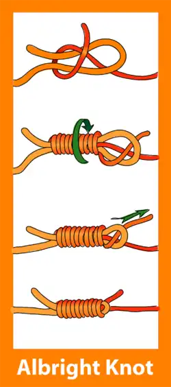
    The Albright special [1] or Albright knot is a bend used in angling. It is a strong knot used to tie two different diameters of line together, for instance to tie monofilament to braid. The Albright is relatively smooth and passes through guides when required. Some anglers coat the knot with a rubber based cement to make it even smoother and more secure.

    As this is an angling bend, it is appropriate for use in fishing line such as monofilament, which is finer, more rigid, and more slippery than ‘conventional’ cords (e.g. braided rope or paracord). Regular knots tied in such cord tend to behave unreliably; hence, one must take additional care when tying many fishing and surgical knots to prevent them from unraveling and spilling. For the Albright special, it is important to wind the turns neatly around the loop of larger line and dress the knot so that each turn sits tight.

    For a more general-purpose bend to join more conventional lines of different diameters, see sheet bend (which, again, can be made more secure by adding turns).

    See also


    References

    1. The complete guide to knots and knot tying — Geoffrey Budworth — p.70 — ISBN 0-7548-0422-4


    External links


    This article is adapted from “Albright special” on Wikipedia, written by its contributors, and used under CC BY-SA 4.0. Text on this page is available under the same licence. Source snapshot: Wikipedia via Kiwix, 2026-07-20.