Category: Knots

  • Matsumoto’s theorem (group theory)

    In group theory, Matsumoto’s theorem, proved by Hideya Matsumoto (1964), gives conditions for two reduced words of a Coxeter group to represent the same element. Sometimes, this is also called Matsumoto’s lemma.[1]

    Statement

    A Coxeter group is a group that admits a presentation G = X R S {\displaystyle G=\langle X\mid R\sqcup S\rangle } {\displaystyle G=\langle X\mid R\sqcup S\rangle }, where X {\displaystyle X} {\displaystyle X} is a set of generators, R {\displaystyle R} {\displaystyle R} is a set of relations of the form x y x y = y x y x {\displaystyle xyxy\ldots =yxyx\ldots } {\displaystyle xyxy\ldots =yxyx\ldots } for x , y X {\displaystyle x,y\in X} {\displaystyle x,y\in X}, where the two sides of the relation are words of same length; and S {\displaystyle S} {\displaystyle S} is the set of relations x 2 = 1 {\displaystyle x^{2}=1} {\displaystyle x^{2}=1} for all x X {\displaystyle x\in X} {\displaystyle x\in X}. The relations in R {\displaystyle R} {\displaystyle R} are sometimes called Artin relations, because the defining relations of an Artin group have this form.

    If two reduced words represent the same element of a Coxeter group, then Matsumoto’s theorem states that the first word can be transformed into the second by repeatedly transforming

    xyxy… to yxyx… (or vice versa).

    In other words: if two reduced words are equivalent in the group, then they are equivalent under the sole Artin relations.

    Applications

    Matsumoto’s theorem implies that there is a natural map (not a group homomorphism) from a Coxeter group to the corresponding braid group, taking any element of the Coxeter group represented by some reduced word in the generators to the same word in the generators of the braid group.

    References

    1. Michel, Patrick Dehornoy, François Digne, Eddy Godelle, Daan Krammer, Jean. “Foundations of Garside Theory | EMS Press”. ems.press. doi:10.4171/139. Retrieved 2025-05-22.{{cite web}}: CS1 maint: multiple names: authors list (link)
    • Matsumoto, Hideya (1964), “Générateurs et relations des groupes de Weyl généralisés”, C. R. Acad. Sci. Paris, 258: 3419–3422, MR 0183818
    • P. Dehornoy et al., “Foundations of Garside theory”, EMS Tracts in Mathematics, 22, Eur. Math. Soc., Zürich, 2015, MR 3362691


    This article is adapted from “Matsumoto's theorem (group theory)” on Wikipedia, written by its contributors, and used under CC BY-SA 4.0. Text on this page is available under the same licence. Source snapshot: Wikipedia via Kiwix, 2026-07-20.
  • 74 knot

    74
    74 knot
    Arf invariant 0
    Braid length 9
    Braid no. 4
    Bridge no. 2
    Crosscap no. 3
    Crossing no. 7
    Genus 1
    Hyperbolic volume 5.13794
    Stick no. 9
    Unknotting no. 2
    Conway notation [313]
    A–B notation 74
    Dowker notation 6, 10, 12, 14, 4, 2, 8
    Last / Next 73 / 75
    Other
    alternating, hyperbolic, prime, reversible, tricolorable

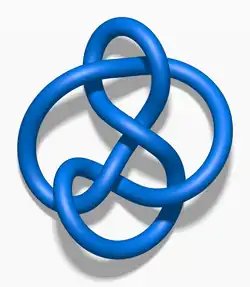
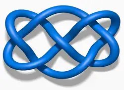
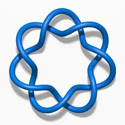
    In mathematical knot theory, 74 is the name of a 7-crossing knot which can be visually depicted in a highly-symmetric form, and so appears in the symbolism and/or artistic ornamentation of various cultures.

    Visual representations

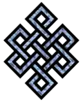
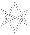
    The interlaced version of the simplest form of the Endless knot symbol of Buddhism is topologically equivalent to the 74 knot (though it appears to have nine crossings), as is the interlaced version of the unicursal hexagram of occultism.[1] (However, the endless knot symbol has more complex forms not equivalent to 74, and both the endless knot and unicursal hexagram can appear in non-interlaced versions, in which case they are not knots at all.)

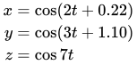
    The 74 knot is a Lissajous knot, representable for example by the parametric equation[2]

    x = cos ( 2 t + 0.22 ) y = cos ( 3 t + 1.10 ) z = cos 7 t {\displaystyle {\begin{aligned}x&=\cos(2t+0.22)\\y&=\cos(3t+1.10)\\z&=\cos 7t\end{aligned}}} {\displaystyle {\begin{aligned}x&=\cos(2t+0.22)\\y&=\cos(3t+1.10)\\z&=\cos 7t\end{aligned}}}
    • One form of the Endless knot of Buddhism
      One form of the Endless knot of Buddhism
    • Interwoven unicursal hexagram.
      Interwoven unicursal hexagram.
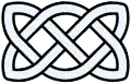
    • 74 knot in Celtic artistic form, also found in some Hausa embroideries.
      74 knot in Celtic artistic form, also found in some Hausa embroideries.[3]
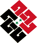
    • A 74 knot combined with the Syrian flag is used as a logo by the National Coordination Committee for Democratic Change.
      A 74 knot combined with the Syrian flag is used as a logo by the National Coordination Committee for Democratic Change.

    Example

    Sources

    1. 7_4“, The Knot Atlas.
    2. Lamm, C. (1997). “There are infinitely many Lissajous knots”. Manuscripta Mathematica. 93: 29–37. doi:10.1007/BF02677455. S2CID 123288245.
    3. Celtic Art: The Methods of Construction by George Bain, p. 27 (ISBN 0-486-22923-8)

    This article is adapted from “74 knot” on Wikipedia, written by its contributors, and used under CC BY-SA 4.0. Text on this page is available under the same licence. Source snapshot: Wikipedia via Kiwix, 2026-07-20.
  • Marudai

    Marudai

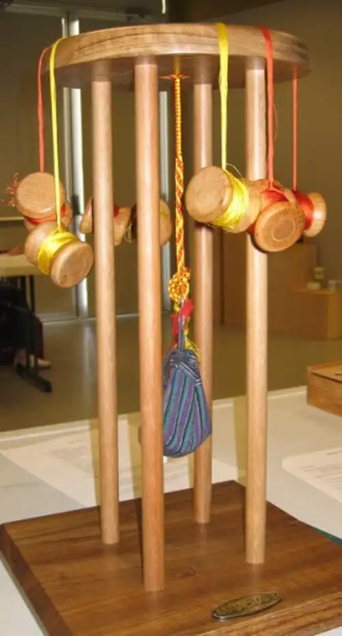
    A marudai (丸台, lit.round stand) is the most common of the traditional frames used for making kumihimo, a type of Japanese braid.[1]

    Etymology

    The marudai is generally made of a close-grained wood and consists of a round disk (kagami or “mirror”)[1] with a hole in the center, supported by four legs set in a base. The Japanese style marudai is often about 16 in (41 cm) high and is used while kneeling or when placed on a table. The Western style 26 in (66 cm) marudai allows the braider to sit in a chair to braid.

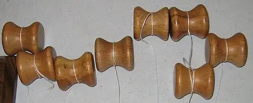
    The warp threads that form the braid are wound around weighted bobbins called tama (lit.egg).[1] Tama were once made of clay, but now are most commonly wood filled with lead. The weight of the tama maintains even tension on the warp threads, and is balanced by a bag of counterweights called omori[1] that is attached to the base of the braid.

    Modern braiders often replace the marudai with a foam disk with numbered slots that tightly grip the warp threads to maintain warp tension, so that weighted bobbins are not needed; instead, flexible plastic bobbins are used to prevent tangling of the threads. Unlike kumihimo disks, marudai have no indication of where the thread should be placed; it is done freehand.

    Related terms

    • Kagami – “Mirror”, the polished wooden top disk of the marudai.[1]
    • Kongō Gumi – a class of patterns for round cord all involving eight threads folded in half for a total of sixteen strands. In clockwise order, each bobbins is moved to the opposite side. When different combinations of thread color are used, many interesting patterns emerge, including diagonal stripes, diamonds on a background, triangles resembling hearts, and tiny six-petalled flowers. Kongō Gumi is named for the venerable Kongō Gumi company of Japan, the oldest known company in the world.
    • Kumihimo or kumi himo – Japanese for “gathered threads”.
    • Obi – the broad cloth sash worn with kimono; kumihimo braids are often used as obijime, worn on top of the obi.
    • Obijime – the cord used to fasten the obi securely in some obi styles. Usually one string of kumihimo is tied around the obi securely, and an accessory called the obidome is often added in front for decoration.
    • Omori – Counterweights used in kumihimo braiding.[1]
    • Takadai – a rectangular or square frame for kumihimo.
    • Tama – little spools. The thread is kept from unwinding by passing the thread under itself, forming a loop around the tama.
    • True silk – a hollow fiber with a rough surface that resists slipping past the loop unless gently pulled. For synthetic fibers, a flexible plastic “clamshell” bobbin may be preferable.
    Several small wooden bobbins, each with a length of thread tied around them.
    A number of tama in use.
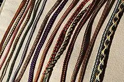
    Several lengths of colourfully-woven braids on a cream background.
    Example kumihimo of several different styles.

    Further reading

    • Yamaoka, Kazuharu Issei. (1975) Domyo no kimihimo : marudai, yotsu-uchidai [Domyo style kumihimo]. Tokyo : Shufunotomo Publication (Handicraft series). OCLC 703820275, JPNO 75076336 (in Japanese)
    • Kyōto Kimono Gakuin. (1979) A Step to kimono and kumihimo. Pasadena, Calif: International College of California. OCLC 5658813.
    • Carey, Jacqui. (1994) Creative Kumihimo. Torquay: Devonshire Press. ISBN 0952322501, 9780952322504, OCLC 888120089.
    • Tada, Makiko. (1996) Andesu No Kumihimo: Kādo to Marudai. [Andean sling braids]. (Kumihimo sōran series, 2) Hino : Tekusuto. 2nd ed., (in Japanese) with some English. ISBN 4925252127, 9784925252126, OCLC 977659717 .
    • Carey, Jacqui. (1997) The Craft of Kumihimo. New York: Midpoint Trade Books, In. ISBN 9780855328283, 0855328282, OCLC 903504434.
    • Carey, Jacqui. (1997) Beginner’s Guide to Braiding, the Craft of Kumihimo. Tunbridge Wells : Search Press. ISBN 0855328282, 9780855328283, OCLC 472775122
    • Tada, Makiko (2008). Tada Makiko Kumihimo-ten : dento no bi to sentan gijutsu [Makiko Tada kumihimo show : traditional beauty and the latest technics]. Naruse Memorial Hall (ed). Tokyo : Japan Women’s College (Tsukuru series 5). NCID BB19346894. (in Japanese)
    • Sakai, Aiko; Tada, Makiko. E o mite wakaru kumihimo : Tanoshiku dekiru marudai kakudai ayadake-dai [Visual guide to kumihimo : practice on marudai, kakudai, and ayadake-dai with fun], Japan Vogue, OCLC 676423318. (in Japanese)
    • Owen, Rodrick. (1995) Braids: 250 Patterns from Japan, Peru & Beyond. Loveland, Colo. : Interweave Press, ISBN 1883010063, 9781883010065, OCLC 31754981. Softcover ed., Berkeley, CA : Lacis, 2004. OCLC 79431006
    • Tada, Makiko. (April 2014) Marudai braids 120.(Comprehensive treatise of braids 1), 3rd ed., Hino  : Tekusuto. (in Japanese) with some English. OCLC 676423383
    • Chottikampon K.; Mathurosemontri S.; Marui H.; Sirisuwan P.; Inoda M., et al. (2015) Comparison of braiding skills between expert and non-experts by eye’s movement measurement. Lecture Notes in Computer Science (including subseries Lecture Notes in Artificial Intelligence and Lecture Notes in Bioinformatics) 9184 (2015): 14-23 ISSN 0302-9743, OCLC 5932476964
    • Tada, Makiko. (2017). Utsukushii kumihimo to komono no reshipi: marudai de tsukuru honkakuteki na kumihimo o mijika na dōgu de yasashiku kawaiku. [Beautiful kumihimo recipes for marudai you braid with everyday tools, fun and pretty] Tōkyō : Nihon Bungeisha. ISBN 9784537214901, 4537214902, OCLC 995846156. (in Japanese)

    Footnotes

    References

    1. 1 2 3 4 5 6 Owen, Rodrick (1931-) (2004). Braids : 250 patterns from Japan, Peru & beyond. Berkeley, California: Lacis. ISBN 1893063089. OCLC 79431006.{{cite book}}: CS1 maint: numeric names: authors list (link)


    This article is adapted from “Marudai” on Wikipedia, written by its contributors, and used under CC BY-SA 4.0. Text on this page is available under the same licence. Source snapshot: Wikipedia via Kiwix, 2026-07-20.
  • 71 knot

    71 knot
    71 knot
    Arf invariant 0
    Braid length 7
    Braid no. 2
    Bridge no. 2
    Crosscap no. 1
    Crossing no. 7
    Genus 3
    Hyperbolic volume 0
    Stick no. 9
    Unknotting no. 3
    Conway notation [7]
    A–B notation 71
    Dowker notation 8, 10, 12, 14, 2, 4, 6
    Last / Next 63 / 72
    Other
    alternating, torus, fibered, prime, reversible

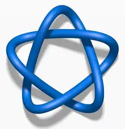
    In knot theory, the 71 knot, also known as the septoil knot, the septafoil knot, or the (7, 2)-torus knot, is one of seven prime knots with crossing number seven. It is the simplest torus knot after the trefoil and cinquefoil. This knot is used to construct the simplest counterexample to the conjecture that the unknotting number is additive under connected sum.[1][2]

    Properties

    The 71 knot is invertible but not amphichiral. Its Alexander polynomial is

    Δ ( t ) = t 3 t 2 + t 1 + t 1 t 2 + t 3 , {\displaystyle \Delta (t)=t^{3}-t^{2}+t-1+t^{-1}-t^{-2}+t^{-3},\,} {\displaystyle \Delta (t)=t^{3}-t^{2}+t-1+t^{-1}-t^{-2}+t^{-3},\,}

    its Conway polynomial is

    ( z ) = z 6 + 5 z 4 + 6 z 2 + 1 , {\displaystyle \nabla (z)=z^{6}+5z^{4}+6z^{2}+1,\,} {\displaystyle \nabla (z)=z^{6}+5z^{4}+6z^{2}+1,\,}

    and its Jones polynomial is

    V ( q ) = q 3 + q 5 q 6 + q 7 q 8 + q 9 q 10 . {\displaystyle V(q)=q^{-3}+q^{-5}-q^{-6}+q^{-7}-q^{-8}+q^{-9}-q^{-10}.\,} {\displaystyle V(q)=q^{-3}+q^{-5}-q^{-6}+q^{-7}-q^{-8}+q^{-9}-q^{-10}.\,}[3]

    Example

    See also

    • Heptagram

    References

    1. Brittenham, Mark; Hermiller, Susan (2025). “Unknotting number is not additive under connected sum”. arXiv:2506.24088 [math.GT].
    2. Sloman, Leila (2025-09-22). “A Simple Way To Measure Knots Has Come Unraveled”. Quanta Magazine. Retrieved 2025-09-22.
    3. 7_1“, The Knot Atlas.


    This article is adapted from “71 knot” on Wikipedia, written by its contributors, and used under CC BY-SA 4.0. Text on this page is available under the same licence. Source snapshot: Wikipedia via Kiwix, 2026-07-20.
  • Marlinespike hitch

    Marlinespike hitch
    Marlinespike hitch
    Names Marlinespike hitch, marlingspike hitch, boat knot
    Category Hitch
    Related Overhand slip knot, stein knot
    Releasing Non-jamming
    Typical use Pulling heavily on rope or twine, historically used by sailors
    Caveat Intended as temporary hitch; not stable unless loaded
    ABoK #559, #1186, #1789, #1880, #2030, #7, #43

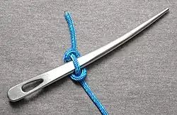
    The marlinespike hitch is a temporary knot used to attach a rod to a rope in order to form a handle.[1] This allows more tension than could be produced comfortably by gripping the rope with the hands alone. It is useful when tightening knots and for other purposes in ropework.

    As the name suggests, the type of rod traditionally used with this hitch is a marlinespike. The advantages of this hitch over others which might serve the purpose are its quickness of tying and ease of releasing. Topologically it is a form of the noose, but in practice this hitch is not allowed to collapse into that shape. When it does capsize into a traditional noose, it can jam against the rod, making it much more difficult to release.[2]

    The hitch is frequently used by hammock campers to attach adjustable rope slings (“whoopie slings”) to the webbing straps that are used to attach hammocks to trees.

    By passing the working end through the marlinespike hitch, this knot can be used as an alternative method of tying the Bowline knot. Passing through in the opposite direction will give you the Cowboy bowline (also known as the left-hand bowline, Dutch marine bowline or winter bowline).

    Marlinespike hitch
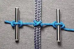
    A constrictor knot prepared for tightening using two rods and marlinespike hitches

    Tying

    Below is a basic method of tying. The knot can also be made by using the rod itself to form the loop, but the tying method does not affect the performance of the resulting hitch.

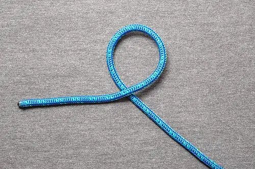
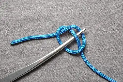
    Begin with an overhand loop, that is, a loop in which the working part passes over the standing part:
    Marlinespike hitch

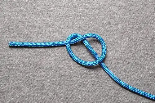
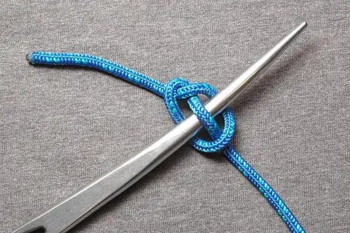
    Fold the loop over the working part, towards the standing part such that the standing part is visible through the center of the loop:
    Marlinespike hitch
    In stiffer material the first two steps can be accomplished in a single motion by twisting the working part with the fingers until a loop forms and flops over the standing part.

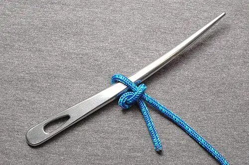
    Use the rod to snag a bight of the standing part through the loop, that is, pass the rod over the near side of the loop, under the standing part and then over the far side of the loop:
    Marlinespike hitch

    Before tensioning, excess slack can be removed by pulling simultaneously on both the working and standing parts:
    Marlinespike hitch
    In actual use the hitch should be loaded only from the standing side.

    Undesirable capsized form

    If the working end is loaded rather than the standing part, the knot will capsize into an overhand noose:
    Marlinespike hitch
    While this form may still hold when the standing part is subsequently loaded, it can jam badly against the rod. This is especially troublesome if the rod is not tapered.

    See also

    • Marlinespike seamanship

    References

    1. Clifford W. Ashley, The Ashley Book of Knots (New York: Doubleday, 1944), 330.
    2. Ashley, 303, 305.

    This article is adapted from “Marlinespike hitch” on Wikipedia, written by its contributors, and used under CC BY-SA 4.0. Text on this page is available under the same licence. Source snapshot: Wikipedia via Kiwix, 2026-07-20.
  • 63 knot

    63 knot
    63 knot
    Arf invariant 1
    Braid length 6
    Braid no. 3
    Bridge no. 2
    Crosscap no. 3
    Crossing no. 6
    Genus 2
    Hyperbolic volume 5.69302
    Stick no. 8
    Unknotting no. 1
    Conway notation [2112]
    A–B notation 63
    Dowker notation 4, 8, 10, 2, 12, 6
    Last / Next 62 / 71
    Other
    alternating, hyperbolic, fibered, prime, fully amphichiral

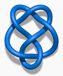
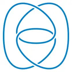
    In knot theory, the 63 knot is one of three prime knots with crossing number six, the others being the stevedore knot and the 62 knot. It is alternating, hyperbolic, and fully amphichiral.
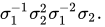
    It can be written as the braid word

    σ 1 1 σ 2 2 σ 1 2 σ 2 . {\displaystyle \sigma _{1}^{-1}\sigma _{2}^{2}\sigma _{1}^{-2}\sigma _{2}.\,} {\displaystyle \sigma _{1}^{-1}\sigma _{2}^{2}\sigma _{1}^{-2}\sigma _{2}.\,}[1]

    Symmetry

    Like the figure-eight knot, the 63 knot is fully amphichiral. This means that the 63 knot is amphichiral,[2] meaning that it is indistinguishable from its own mirror image. In addition, it is also invertible, meaning that orienting the curve in either direction yields the same oriented knot.

    Invariants

    The Alexander polynomial of the 63 knot is

    Δ ( t ) = t 2 3 t + 5 3 t 1 + t 2 , {\displaystyle \Delta (t)=t^{2}-3t+5-3t^{-1}+t^{-2},\,} {\displaystyle \Delta (t)=t^{2}-3t+5-3t^{-1}+t^{-2},\,}

    Conway polynomial is

    ( z ) = z 4 + z 2 + 1 , {\displaystyle \nabla (z)=z^{4}+z^{2}+1,\,} {\displaystyle \nabla (z)=z^{4}+z^{2}+1,\,}

    Jones polynomial is

    V ( q ) = q 3 + 2 q 2 2 q + 3 2 q 1 + 2 q 2 q 3 , {\displaystyle V(q)=-q^{3}+2q^{2}-2q+3-2q^{-1}+2q^{-2}-q^{-3},\,} {\displaystyle V(q)=-q^{3}+2q^{2}-2q+3-2q^{-1}+2q^{-2}-q^{-3},\,}

    and the Kauffman polynomial is

    L ( a , z ) = a z 5 + z 5 a 1 + 2 a 2 z 4 + 2 z 4 a 2 + 4 z 4 + a 3 z 3 + a z 3 + z 3 a 1 + z 3 a 3 3 a 2 z 2 3 z 2 a 2 6 z 2 a 3 z 2 a z 2 z a 1 z a 3 + a 2 + a 2 + 3. {\displaystyle L(a,z)=az^{5}+z^{5}a^{-1}+2a^{2}z^{4}+2z^{4}a^{-2}+4z^{4}+a^{3}z^{3}+az^{3}+z^{3}a^{-1}+z^{3}a^{-3}-3a^{2}z^{2}-3z^{2}a^{-2}-6z^{2}-a^{3}z-2az-2za^{-1}-za^{}-3+a^{2}+a^{-2}+3.\,} {\displaystyle L(a,z)=az^{5}+z^{5}a^{-1}+2a^{2}z^{4}+2z^{4}a^{-2}+4z^{4}+a^{3}z^{3}+az^{3}+z^{3}a^{-1}+z^{3}a^{-3}-3a^{2}z^{2}-3z^{2}a^{-2}-6z^{2}-a^{3}z-2az-2za^{-1}-za^{}-3+a^{2}+a^{-2}+3.\,} [3]

    The 63 knot is a hyperbolic knot, with its complement having a volume of approximately 5.69302.

    References

    1. “6_3 knot – Wolfram|Alpha”.
    2. Weisstein, Eric W. “Amphichiral Knot”. MathWorld. Accessed: May 12, 2014.
    3. 6_3“, The Knot Atlas.


    This article is adapted from “63 knot” on Wikipedia, written by its contributors, and used under CC BY-SA 4.0. Text on this page is available under the same licence. Source snapshot: Wikipedia via Kiwix, 2026-07-20.
  • 62 knot

    62 knot
    62 knot
    Arf invariant 1
    Braid length 6
    Braid no. 3
    Bridge no. 2
    Crosscap no. 2
    Crossing no. 6
    Genus 2
    Hyperbolic volume 4.40083
    Stick no. 8
    Unknotting no. 1
    Conway notation [312]
    A–B notation 62
    Dowker notation 4, 8, 10, 12, 2, 6
    Last / Next 61 / 63
    Other
    alternating, hyperbolic, fibered, prime, reversible

    In knot theory, the 62 knot is one of three prime knots with crossing number six, the others being the stevedore knot and the 63 knot. This knot is sometimes referred to as the Miller Institute knot,[1] because it appears in the logo[2] of the Miller Institute for Basic Research in Science at the University of California, Berkeley.

    The 62 knot is invertible but not amphichiral. Its Alexander polynomial is

    Δ ( t ) = t 2 + 3 t 3 + 3 t 1 t 2 , {\displaystyle \Delta (t)=-t^{2}+3t-3+3t^{-1}-t^{-2},\,} {\displaystyle \Delta (t)=-t^{2}+3t-3+3t^{-1}-t^{-2},\,}

    its Conway polynomial is

    ( z ) = z 4 z 2 + 1 , {\displaystyle \nabla (z)=-z^{4}-z^{2}+1,\,} {\displaystyle \nabla (z)=-z^{4}-z^{2}+1,\,}

    and its Jones polynomial is

    V ( q ) = q 1 + 2 q 1 2 q 2 + 2 q 3 2 q 4 + q 5 . {\displaystyle V(q)=q-1+2q^{-1}-2q^{-2}+2q^{-3}-2q^{-4}+q^{-5}.\,} {\displaystyle V(q)=q-1+2q^{-1}-2q^{-2}+2q^{-3}-2q^{-4}+q^{-5}.\,}[3]

    The 62 knot is a hyperbolic knot, with its complement having a volume of approximately 4.40083.

    Surface

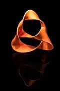
    • Surface of knot 6.2
      Surface of knot 6.2

    Example

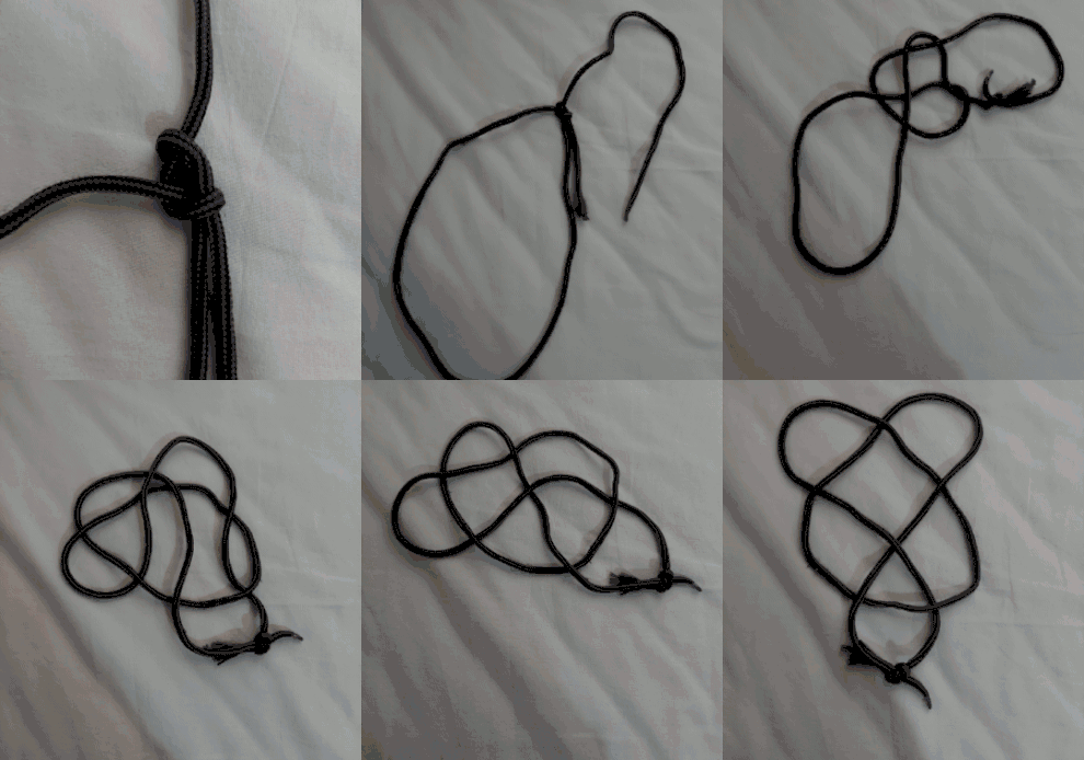
    Ways to assemble of knot 6.2

    • Example 1
    • Example 2

    If a bowline is tied and the two free ends of the rope are brought together in the simplest way, the knot obtained is the 62 knot. The sequence of necessary moves are depicted here:

    • From a bowline (ends connected) to the 6₂ knot
      From a bowline (ends connected) to the 6₂ knot

    References


    This article is adapted from “62 knot” on Wikipedia, written by its contributors, and used under CC BY-SA 4.0. Text on this page is available under the same licence. Source snapshot: Wikipedia via Kiwix, 2026-07-20.
  • Markov theorem

    Markov theorem
    Braid closure

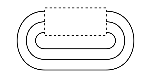
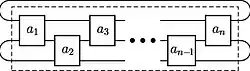
    In mathematics the Markov theorem gives necessary and sufficient conditions for two braids to have closures that are equivalent knots or links. The conditions are stated in terms of the group structures on braids.

    Braids are algebraic objects described by diagrams; the relation to topology is given by Alexander’s theorem which states that every knot or link in three-dimensional Euclidean space is the closure of a braid. The Markov theorem, proved by Russian mathematician Andrei Andreevich Markov Jr.[1] describes the elementary moves generating the equivalence relation on braids given by the equivalence of their closures.

    More precisely Markov’s theorem can be stated as follows:[2][3] given two braids represented by elements β n , β m {\displaystyle \beta _{n},\beta _{m}’} {\displaystyle \beta _{n},\beta _{m}'} in the braid groups B n , B m {\displaystyle B_{n},B_{m}} {\displaystyle B_{n},B_{m}}, their closures are equivalent links if and only if β m {\displaystyle \beta _{m}’} {\displaystyle \beta _{m}'} can be obtained from applying to β n {\displaystyle \beta _{n}} {\displaystyle \beta _{n}} a sequence of the following operations:

    1. conjugating β n {\displaystyle \beta _{n}} {\displaystyle \beta _{n}} in B n {\displaystyle B_{n}} {\displaystyle B_{n}};
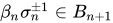
    2. replacing β n {\displaystyle \beta _{n}} {\displaystyle \beta _{n}} by β n σ n ± 1 B n + 1 {\displaystyle \beta _{n}\sigma _{n}^{\pm 1}\in B_{n+1}} {\displaystyle \beta _{n}\sigma _{n}^{\pm 1}\in B_{n+1}} (here σ i {\displaystyle \sigma _{i}} {\displaystyle \sigma _{i}} are the standard generators of the braid groups; geometrically this amounts to adding a strand to the right of the braid diagram and twisting it once with the (previously) last strand);
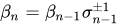
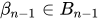
    3. the inverse of the previous operation (if β n = β n 1 σ n 1 ± 1 {\displaystyle \beta _{n}=\beta _{n-1}\sigma _{n-1}^{\pm 1}} {\displaystyle \beta _{n}=\beta _{n-1}\sigma _{n-1}^{\pm 1}} with β n 1 B n 1 {\displaystyle \beta _{n-1}\in B_{n-1}} {\displaystyle \beta _{n-1}\in B_{n-1}} replace with β n 1 {\displaystyle \beta _{n-1}} {\displaystyle \beta _{n-1}}).

    In 1974 American mathematician Joan Birman published a monograph, Braids, Links, and Mapping Class Groups, based on a graduate course she taught as a visiting professor at Princeton University in 1971–72; this book contains the first complete proof of the Markov theorem.[4]

    References

    1. A. A. Markov Jr., Über die freie Äquivalenz der geschlossenen Zöpfe
    2. Birman, Joan (1974). Braids, Links, and Mapping Class Groups. Annals of Mathematics Studies. Vol. 82. Princeton University Press., Theorem 2.3 on p. 51
    3. Kauffman, Louis (1991). Knots and Physics. World Scientific., p.95
    4. Margalit, Dan (2019). “The Mathematics of Joan Birman” (PDF). AMS Notices. 66 (3).

    This article is adapted from “Markov theorem” on Wikipedia, written by its contributors, and used under CC BY-SA 4.0. Text on this page is available under the same licence. Source snapshot: Wikipedia via Kiwix, 2026-07-20.
  • Magnus hitch

    Magnus hitch
    Names Magnus hitch, Adjustable hitch
    Category Hitch
    Related Taut-line hitch, Rolling hitch, Two half-hitches, Trucker’s hitch, Adjustable grip hitch
    ABoK #1736, #1857

    The magnus hitch is a knot similar to a rolling hitch or clove hitch, used to tie a rope or line to a pole, spar, or another line. It is tied similarly to a rolling hitch but with the final hitch in the opposite direction. It can be more tricky to snug up, since both lines emerge from the same side of the hitch, but it has less tendency to twist under load.

    Tying

    To tie a magnus hitch:

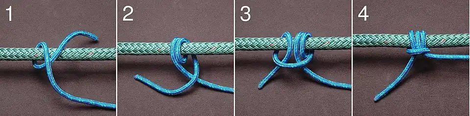
    1. Start with a turn around the object. Bring the working end towards the direction of pull and between the standing part and the object.
    2. Make another wrap around the object, completing a round turn. The wraps of the round turn should progress towards the desired direction of pull. Bring the working end out over the standing part away from the direction of pull.
    3. Complete with a half hitch, moving around the object in the opposite direction as the first turns, as for a cow hitch.
    4. Dress by snugging the hitch around the object before applying load, away from the tail of the hitch.
    Magnus hitch

    See also

    References


    This article is adapted from “Magnus hitch” on Wikipedia, written by its contributors, and used under CC BY-SA 4.0. Text on this page is available under the same licence. Source snapshot: Wikipedia via Kiwix, 2026-07-20.
  • 2-bridge knot

    2-bridge knot
    Schematic picture of a 2-bridge knot.
    Bridge number 2
    2-bridge knot
    31
    2-bridge knot
    51
    2-bridge knot
    63
    2-bridge knot
    71

    In the mathematical field of knot theory, a 2-bridge knot is a knot which can be regular isotoped so that the natural height function given by the z-coordinate has only two maxima and two minima as critical points. Equivalently, these are the knots with bridge number 2, the smallest possible bridge number for a nontrivial knot. Every nontrivial knot with up to seven crossings is a 2-bridge knot. The simplest knots with a bridge number of 3 have eight crossings. Of the 1,701,936 knots with up to sixteen crossings, 5,546 are 2-bridge knots.[1]

    Other names for 2-bridge knots are rational knots, 4-plats, and Viergeflechte (German for four braids). 2-bridge links are defined similarly as above, but each component will have one min and max. 2-bridge knots were classified by Horst Schubert, using the fact that the 2-sheeted branched cover of the 3-sphere over the knot is a lens space.

    Schubert normal form

    The names rational knot and rational link were coined by John Conway who defined them as arising from numerator closures of rational tangles.
    This definition can be used to give a bijection between the set of 2-bridge links and the set of rational numbers; the rational number associated to a given link is called
    the Schubert normal form of the link (as this invariant was first defined by Schubert[2]), and is precisely the fraction associated to the rational tangle whose numerator closure gives the link.[3]:chapter 10

    Further reading

    • Louis H. Kauffman, Sofia Lambropoulou: On the classification of rational knots, L’ Enseignement Mathématique, 49:357410 (2003). preprint available at arxiv.org
    • C. C. Adams, The Knot Book: An elementary introduction to the mathematical theory of knots. American Mathematical Society, Providence, RI, 2004. xiv+307 pp. ISBN 0-8218-3678-1

    References

    1. De Wit, David (2007). “THE 2-BRIDGE KNOTS OF UP TO 16 CROSSINGS” (PDF). Journal of Knot Theory and Its Ramifications. 16 (08): 997–1019. doi:10.1142/S021821650700566X. ISSN 0218-2165. Retrieved 2025-09-06.
    2. Schubert, Horst (1956). “Knoten mit zwei Brücken”. Mathematische Zeitschrift. 65: 133–170. doi:10.1007/bf01473875.
    3. Purcell, Jessica (2020). Hyperbolic knot theory. American Mathematical Society. ISBN 978-1-4704-5499-9.

    External links


    This article is adapted from “2-bridge knot” on Wikipedia, written by its contributors, and used under CC BY-SA 4.0. Text on this page is available under the same licence. Source snapshot: Wikipedia via Kiwix, 2026-07-20.