Category: Knots

  • Connected sum

    Connected sum
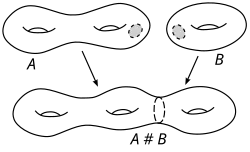
    Illustration of connected sum.

    In mathematics, specifically in topology, the operation of connected sum is a geometric modification on manifolds. Its effect is to join two given manifolds together near a chosen point on each. This construction plays a key role in the classification of closed surfaces.

    More generally, one can also join manifolds together along identical submanifolds; this generalization is often called the fiber sum.

    There is also a closely related notion of a connected sum on knots, called the knot sum or composition of knots.

    Connected sum at a point

    A connected sum of two m-dimensional manifolds is a manifold formed by deleting a ball inside each manifold and gluing together the resulting boundary spheres.

    If both manifolds are oriented, there is a unique connected sum defined by having the gluing map reverse orientation. Although the construction uses the choice of the balls, the result is unique up to homeomorphism. One can also make this operation work in the smooth category, and then the result is unique up to diffeomorphism. There are subtle problems in the smooth case: not every diffeomorphism between the boundaries of the spheres gives the same composite manifold, even if the orientations are chosen correctly. For example, Milnor showed that two 7-cells can be glued along their boundary so that the result is an exotic sphere homeomorphic but not diffeomorphic to a 7-sphere.

    However, there is a canonical way to choose the gluing of M 1 {\displaystyle M_{1}} {\displaystyle M_{1}} and M 2 {\displaystyle M_{2}} {\displaystyle M_{2}} which gives a unique well-defined connected sum.[1] Choose embeddings i 1 : D n M 1 {\displaystyle i_{1}:D_{n}\rightarrow M_{1}} {\displaystyle i_{1}:D_{n}\rightarrow M_{1}} and i 2 : D n M 2 {\displaystyle i_{2}:D_{n}\rightarrow M_{2}} {\displaystyle i_{2}:D_{n}\rightarrow M_{2}} so that i 1 {\displaystyle i_{1}} {\displaystyle i_{1}} preserves orientation and i 2 {\displaystyle i_{2}} {\displaystyle i_{2}} reverses orientation. Now obtain M 1 # M 2 {\displaystyle M_{1}\mathbin {\#} M_{2}} {\displaystyle M_{1}\mathbin {\#} M_{2}} from the disjoint sum

    ( M 1 i 1 ( 0 ) ) ( M 2 i 2 ( 0 ) ) {\displaystyle (M_{1}-i_{1}(0))\sqcup (M_{2}-i_{2}(0))} {\displaystyle (M_{1}-i_{1}(0))\sqcup (M_{2}-i_{2}(0))}

    by identifying i 1 ( t u ) {\displaystyle i_{1}(tu)} {\displaystyle i_{1}(tu)} with i 2 ( ( 1 t ) u ) {\displaystyle i_{2}((1-t)u)} {\displaystyle i_{2}((1-t)u)} for each unit vector u S n 1 {\displaystyle u\in S^{n-1}} {\displaystyle u\in S^{n-1}} and each 0 < t < 1 {\displaystyle 0<t<1} {\displaystyle 0<t<1}. Choose the orientation for M 1 # M 2 {\displaystyle M_{1}\mathbin {\#} M_{2}} {\displaystyle M_{1}\mathbin {\#} M_{2}} which is compatible with M 1 {\displaystyle M_{1}} {\displaystyle M_{1}} and M 2 {\displaystyle M_{2}} {\displaystyle M_{2}}. The fact that this construction is well-defined depends crucially on the disc theorem, which is not at all obvious. For further details, see Kosinski, Differential Manifolds.[2]

    The operation of connected sum is denoted by # {\displaystyle \#} {\displaystyle \#}.

    The operation of connected sum has the sphere S m {\displaystyle S^{m}} {\displaystyle S^{m}} as an identity; that is, M # S m {\displaystyle M\mathbin {\#} S^{m}} {\displaystyle M\mathbin {\#} S^{m}} is homeomorphic (or diffeomorphic) to M {\displaystyle M} {\displaystyle M}.

    The classification of closed surfaces, a foundational and historically significant result in topology, states that any closed surface can be expressed as the connected sum of a sphere with some number g {\displaystyle g} {\displaystyle g} of tori and some number k {\displaystyle k} {\displaystyle k} of real projective planes.

    Connected sum along a submanifold

    The connected sum can be defined along a submanifold.[3]:§1

    Let M 1 {\displaystyle M_{1}} {\displaystyle M_{1}} and M 2 {\displaystyle M_{2}} {\displaystyle M_{2}} be two smooth, oriented manifolds of equal dimension and V {\displaystyle V} {\displaystyle V} a smooth, closed, oriented manifold, embedded as a submanifold into both M 1 {\displaystyle M_{1}} {\displaystyle M_{1}} and M 2 . {\displaystyle M_{2}.} {\displaystyle M_{2}.} Suppose furthermore that there exists an isomorphism of normal bundles

    ψ : N M 1 V N M 2 V {\displaystyle \psi :N_{M_{1}}V\to N_{M_{2}}V} {\displaystyle \psi :N_{M_{1}}V\to N_{M_{2}}V}

    that reverses the orientation on each fiber. Then ψ {\displaystyle \psi } {\displaystyle \psi } induces an orientation-preserving diffeomorphism

    N 1 V N M 1 V V N M 2 V V N 2 V , {\displaystyle N_{1}\setminus V\cong N_{M_{1}}V\setminus V\to N_{M_{2}}V\setminus V\cong N_{2}\setminus V,} {\displaystyle N_{1}\setminus V\cong N_{M_{1}}V\setminus V\to N_{M_{2}}V\setminus V\cong N_{2}\setminus V,}

    where each normal bundle N M i V {\displaystyle N_{M_{i}}V} {\displaystyle N_{M_{i}}V} is diffeomorphically identified with a neighborhood N i {\displaystyle N_{i}} {\displaystyle N_{i}} of V {\displaystyle V} {\displaystyle V} in M i {\displaystyle M_{i}} {\displaystyle M_{i}}, and the map

    N M 1 V V N M 2 V V {\displaystyle N_{M_{1}}V\setminus V\to N_{M_{2}}V\setminus V} {\displaystyle N_{M_{1}}V\setminus V\to N_{M_{2}}V\setminus V}

    is the orientation-reversing diffeomorphic involution

    v v / | v | 2 {\displaystyle v\mapsto v/|v|^{2}} {\displaystyle v\mapsto v/|v|^{2}}

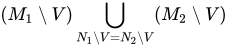
    on normal vectors. The connected sum of M 1 {\displaystyle M_{1}} {\displaystyle M_{1}} and M 2 {\displaystyle M_{2}} {\displaystyle M_{2}} along V {\displaystyle V} {\displaystyle V} is then the space

    ( M 1 V ) N 1 V = N 2 V ( M 2 V ) {\displaystyle (M_{1}\setminus V)\bigcup _{N_{1}\setminus V=N_{2}\setminus V}(M_{2}\setminus V)} {\displaystyle (M_{1}\setminus V)\bigcup _{N_{1}\setminus V=N_{2}\setminus V}(M_{2}\setminus V)}

    obtained by gluing the deleted neighborhoods together by the orientation-preserving diffeomorphism. The sum is often denoted

    ( M 1 , V ) # ( M 2 , V ) . {\displaystyle (M_{1},V)\mathbin {\#} (M_{2},V).} {\displaystyle (M_{1},V)\mathbin {\#} (M_{2},V).}

    Its diffeomorphism type depends on the choice of the two embeddings of V {\displaystyle V} {\displaystyle V} and on the choice of ψ {\displaystyle \psi } {\displaystyle \psi }.

    Loosely speaking, each normal fiber of the submanifold V {\displaystyle V} {\displaystyle V} contains a single point of V {\displaystyle V} {\displaystyle V}, and the connected sum along V {\displaystyle V} {\displaystyle V} is simply the connected sum as described in the preceding section, performed along each fiber. For this reason, the connected sum along V {\displaystyle V} {\displaystyle V} is often called the fiber sum.

    The special case of V {\displaystyle V} {\displaystyle V} a point recovers the connected sum of the preceding section.

    Connected sum along a codimension-two submanifold

    Another important special case occurs when the dimension of V {\displaystyle V} {\displaystyle V} is two less than that of the M i {\displaystyle M_{i}} {\displaystyle M_{i}}. Then the isomorphism ψ {\displaystyle \psi } {\displaystyle \psi } of normal bundles exists whenever their Euler classes are opposite:

    e ( N M 1 V ) = e ( N M 2 V ) . {\displaystyle e\left(N_{M_{1}}V\right)=-e\left(N_{M_{2}}V\right).} {\displaystyle e\left(N_{M_{1}}V\right)=-e\left(N_{M_{2}}V\right).}

    Furthermore, in this case the structure group of the normal bundles is the circle group S O ( 2 ) {\displaystyle SO(2)} {\displaystyle SO(2)}; it follows that the choice of embeddings can be canonically identified with the group of homotopy classes of maps from V {\displaystyle V} {\displaystyle V} to the circle, which in turn equals the first integral cohomology group H 1 ( V ) {\displaystyle H^{1}(V)} {\displaystyle H^{1}(V)}. So the diffeomorphism type of the sum depends on the choice of ψ {\displaystyle \psi } {\displaystyle \psi } and a choice of element from H 1 ( V ) {\displaystyle H^{1}(V)} {\displaystyle H^{1}(V)}.

    A connected sum along a codimension-two V {\displaystyle V} {\displaystyle V} can also be carried out in the category of symplectic manifolds; this elaboration is called the symplectic sum.

    Local operation

    The connected sum is a local operation on manifolds, meaning that it alters the summands only in a neighborhood of V {\displaystyle V} {\displaystyle V}. This implies, for example, that the sum can be carried out on a single manifold M {\displaystyle M} {\displaystyle M} containing two disjoint copies of V {\displaystyle V} {\displaystyle V}, with the effect of gluing M {\displaystyle M} {\displaystyle M} to itself. For example, the connected sum of a 2-sphere at two distinct points of the sphere produces the 2-torus.

    Connected sum of knots

    There is a closely related notion of the connected sum of two knots. In fact, if one regards a knot merely as a 1-manifold, then the connected sum of two knots is just their connected sum as a 1-dimensional manifold. However, the essential property of a knot is not its manifold structure (under which every knot is equivalent to a circle) but rather its embedding into the ambient space. So the connected sum of knots has a more elaborate definition that produces a well-defined embedding, as follows.
    Connected sum
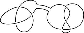
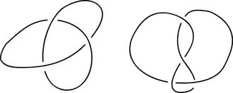
    Consider disjoint planar projections of each knot.
    Connected sum
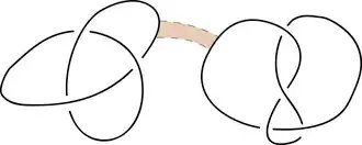
    Find a rectangle in the plane where one pair of sides are arcs along each knot but is otherwise disjoint from the knots.
    Connected sum
    Now join the two knots together by deleting these arcs from the knots and adding the arcs that form the other pair of sides of the rectangle.

    This procedure results in the projection of a new knot, a connected sum (or knot sum, or composition) of the original knots. For the connected sum of knots to be well defined, one has to consider oriented knots in 3-space. To define the connected sum for two oriented knots:

    1. Consider a planar projection of each knot and suppose these projections are disjoint.
    2. Find a rectangle in the plane where one pair of sides are arcs along each knot but is otherwise disjoint from the knots and so that the arcs of the knots on the sides of the rectangle are oriented around the boundary of the rectangle in the same direction.
    3. Now join the two knots together by deleting these arcs from the knots and adding the arcs that form the other pair of sides of the rectangle.

    The resulting connected sum knot inherits an orientation consistent with the orientations of the two original knots, and the oriented ambient isotopy class of the result is well-defined, depending only on the oriented ambient isotopy classes of the original two knots.

    Under this operation, oriented knots in 3-space form a commutative monoid with unique prime factorization, which allows us to define what is meant by a prime knot. Proof of commutativity can be seen by letting one summand shrink until it is very small and then pulling it along the other knot. The unknot is the unit. The two trefoil knots are the simplest prime knots. Higher-dimensional knots can be added by splicing the n {\displaystyle n} {\displaystyle n}-spheres.

    In three dimensions, the unknot cannot be written as the sum of two non-trivial knots. This fact follows from additivity of knot genus; another proof relies on an infinite construction sometimes called the Mazur swindle. In higher dimensions (with codimension at least three), it is possible to get an unknot by adding two nontrivial knots.

    If one does not take into account the orientations of the knots, the connected sum operation is not well-defined on isotopy classes of (nonoriented) knots. To see this, consider two noninvertible knots K, L which are not equivalent (as unoriented knots); for example take the two pretzel knots K = P(3, 5, 7) and L = P(3, 5, 9). Let K+ and K be K with its two inequivalent orientations, and let L+ and L be L with its two inequivalent orientations. There are four oriented connected sums we may form:

    • A = K+ # L+
    • B = K # L
    • C = K+ # L
    • D = K # L+

    The oriented ambient isotopy classes of these four oriented knots are all distinct, and, when one considers ambient isotopy of the knots without regard to orientation, there are two distinct equivalence classes: {A ~ B} and {C ~ D}. To see that A and B are unoriented equivalent, simply note that they both may be constructed from the same pair of disjoint knot projections as above, the only difference being the orientations of the knots. Similarly, one sees that C and D may be constructed from the same pair of disjoint knot projections.

    See also

    Further reading

    • Robert Gompf: A new construction of symplectic manifolds, Annals of Mathematics 142 (1995), 527–595
    • William S. Massey, A Basic Course in Algebraic Topology, Springer-Verlag, 1991. ISBN 0-387-97430-X.

    References

    1. Kervaire and Milnor, Groups of Homotopy Spheres I, Annals of Mathematics Vol 77 No 3 May 1963
    2. Antoni A. Kosinski, Differential Manifolds, Academic Press (1992), reprinted by Dover Publications (2007).
    3. Gompf, Robert E. (November 1995). “A New Construction of Symplectic Manifolds”. The Annals of Mathematics. 142 (3): 527. doi:10.2307/2118554.

    This article is adapted from “Connected sum” on Wikipedia, written by its contributors, and used under CC BY-SA 4.0. Text on this page is available under the same licence. Source snapshot: Wikipedia via Kiwix, 2026-07-20.
  • Clove hitch

    Clove hitch
    Clove hitch
    Category Hitch
    Origin Ancient
    Related Slippery hitch, Two half-hitches, Buntline hitch, Cow hitch, Constrictor knot, Ground-line hitch, Lashings, Snuggle hitch
    Typical use Securing lines running along a series of posts, belaying, starting lashings, weak binding
    Caveat Can spill if the standing part is pulled forcibly in the wrong direction
    ABoK #11, #53, #69, #70, #204, #400, #421, #437, #1176, #1177, #1178, #1179, #1180, #1245, #1773, #1774, #1775, #1776, #1778, #1779, #1814, #2079, #2541, #2542, #2543, #2544, #2546, #2547, #2548
    Instructions https://www.youtube.com/watch?v=pwdZTHu5rTI

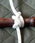
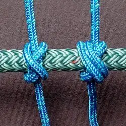
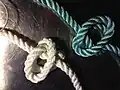
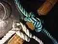
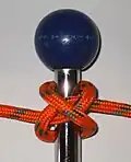
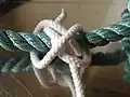
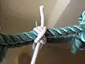
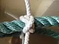
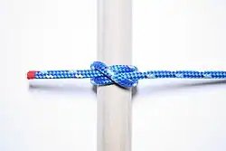
    The clove hitch is an ancient type of knot, made of two successive single hitches[1]:283 tied around an object. It is most effectively used to secure a middle section of rope to an object it crosses over,[1]:213 such as a line on a fencepost. It can also be used as an ordinary hitch, or as a binding knot, but it is not particularly secure in either application.[1]:18,224 It is considered one of the most important knots, alongside the bowline and the sheet bend.

    Although the name clove hitch is given by Falconer in his Dictionary of 1769, the knot is much older, having been tied in ratlines at least as early as the first quarter of the sixteenth century. This is shown in early sculpture and paintings. A round turn is taken with the ratline and then a hitch is added below. The forward end is always the first to be made fast.

    The Ashley Book of Knots[1]:214

    Usage

    This knot is particularly useful where the length of the running end needs to be adjustable, since feeding in rope from either direction will loosen the knot to be tightened at a new position. With certain types of cord, the clove hitch can slip when loaded.[2] In modern climbing rope, the clove hitch will slip to a point, and then stop slipping.[3] When tied around a carabiner, the load should pull on the end closest to its spine.[4] With smaller diameter cords, after being heavily weighted it may become difficult to untie.[2] It is also unreliable when used on a square or rectangular post, rather than round.

    The clove hitch is also commonly used in pioneering to start and finish a lashing such as the traditional square lashing, tripod lashing, round lashing and shear lashing.[5]

    Tying

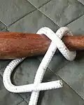
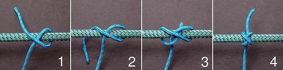
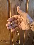
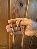
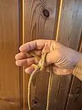
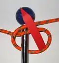
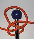
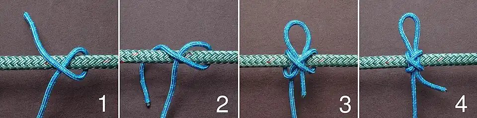
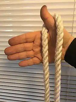
    The clove hitch is tied by first passing the running end of the rope around the spar and back over itself to form an X. The running end then passes around the spar again, under the intersection of the last two turns, and both ends are pulled tight. There are several methods of tying it using both hands[6][7][8][9] or one hand.[10][11][12][13]

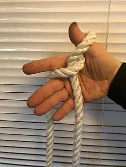
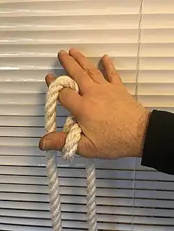
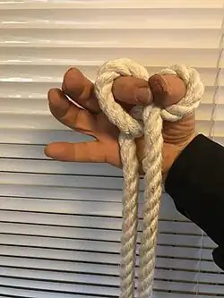
    • 1. The rope hooked by the thumb is let to hang loosely either side.
      1. The rope hooked by the thumb is let to hang loosely either side.
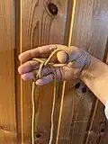
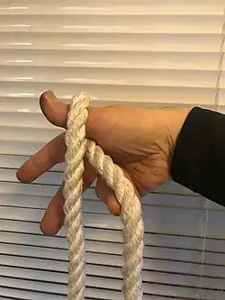
    • 2. The inner rope is pulled back and out using the ring finger.
      2. The inner rope is pulled back and out using the ring finger.
    • 3. The outer rope is pulled in and back using the middle finger.
      3. The outer rope is pulled in and back using the middle finger.
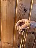
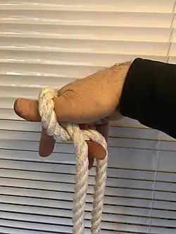
    • 4. The ring and the little finger join the middle finger.
      4. The ring and the little finger join the middle finger.
    • 5. The hand is rotated around the front rope, the index finger gets under then points up.
      5. The hand is rotated around the front rope, the index finger gets under then points up.
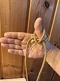
    • 6. The index finger and the thumb are joined to gather the final knot.
      6. The index finger and the thumb are joined to gather the final knot.

    Related knots

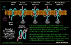
    Clove Family of Constrictor, Bag, Groundline, Strangle.  Knot vs. Hitch.  Purchase as rope taken from system and then can you hold it fast (old sailor terms)
    Clove Family of Constrictor  ABOK#1176, Miller’s/Bag  ABOK#1242, Groundline  ABOK#1243, Strangle  ABOK#1239

    When a turn around an object is made and a clove hitch is tied to the rope’s own standing part, it produces either a buntline hitch or two half-hitches, depending on whether the turns of the clove hitch progress toward or away from the hitched object. Two-half hitches is also the capsized form of a granny knot.[1]:18 The buntline hitch itself is used as a necktie knot called the four-in-hand knot.

    The clove hitch is also a part of a family of binding knots called millers’ knots, which all start with a single hitch tied around an object.

    See also

    References

    1. 1 2 3 4 5 Ashley, Clifford Warren (1944). The Ashley Book of Knots. Knopf Doubleday Publishing Group. ISBN 9780385040259. {{cite book}}: ISBN / Date incompatibility (help)
    2. 1 2 “Clove Hitch – Rope End”. Animated Knots.
    3. Hundal, Geir. “The Climbing Mythbusters”. Geir.com.
    4. “Use and Abuse of the Clove Hitch”. Guide Tricks For Climbers. 2012-12-12. Retrieved 2020-06-02.
    5. “Lashing Information”. www.scoutpioneering.com. 23 February 2013. Retrieved 2013-05-12.
    6. on the working end method on YouTube
    7. with half hitches over object end on YouTube
    8. on the bight arms crossed in one move on YouTube
    9. on the bight with two loops, front one moved back on YouTube
    10. one handed clove hitch on the bight, pinky and thumb on YouTube
    11. one handed clove hitch on the bight both ends hanging on YouTube
    12. one handed clove hitch on the bight to vertical rope on YouTube
    13. one handed clove hitch on the bight into carabiner on YouTube

    External links


    This article is adapted from “Clove hitch” on Wikipedia, written by its contributors, and used under CC BY-SA 4.0. Text on this page is available under the same licence. Source snapshot: Wikipedia via Kiwix, 2026-07-20.
  • Slice knot

    Slice knot
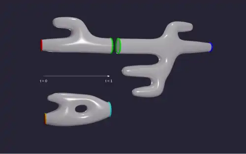
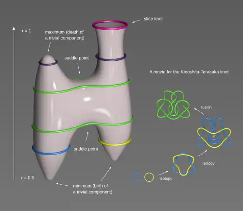
    A smooth slice disk in Morse position, showing minima, saddles and a maximum, and as an illustration a movie for the Kinoshita–Terasaka knot

    A slice knot is a mathematical knot in 3-dimensional space that bounds an embedded disk in 4-dimensional space.

    Definition

    A knot K S 3 {\displaystyle K\subset S^{3}} {\displaystyle K\subset S^{3}} is said to be a topologically slice knot or a smoothly slice knot, if it is the boundary of an embedded disk in the 4-ball B 4 {\displaystyle B^{4}} {\displaystyle B^{4}}, which is locally flat or smooth, respectively. Here we use S 3 = B 4 {\displaystyle S^{3}=\partial B^{4}} {\displaystyle S^{3}=\partial B^{4}}: the 3-sphere S 3 = { x R 4 : | x | = 1 } {\displaystyle S^{3}=\{\mathbf {x} \in \mathbb {R} ^{4}:|\mathbf {x} |=1\}} {\displaystyle S^{3}=\{\mathbf {x} \in \mathbb {R} ^{4}:|\mathbf {x} |=1\}} is the boundary of the four-dimensional ball B 4 = { x R 4 : | x | 1 } . {\displaystyle B^{4}=\{\mathbf {x} \in \mathbb {R} ^{4}:|\mathbf {x} |\leq 1\}.} {\displaystyle B^{4}=\{\mathbf {x} \in \mathbb {R} ^{4}:|\mathbf {x} |\leq 1\}.} Every smoothly slice knot is topologically slice because a smoothly embedded disk is locally flat. Usually, smoothly slice knots are also just called slice. Both types of slice knots are important in 3- and 4-dimensional topology.

    Smoothly slice knots are often illustrated using knots diagrams of ribbon knots and it is an open question whether there are any smoothly slice knots which are not ribbon knots (′Slice-ribbon conjecture′).

    Cone construction

    Slice knot
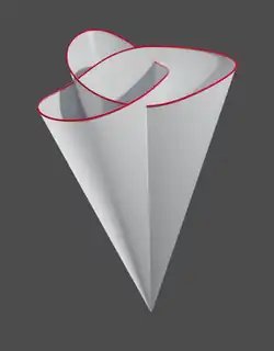
    Cone over the trefoil knot

    The conditions locally-flat or smooth are essential in the definition: For every knot we can construct the cone over the knot which is a disk in the 4-ball with the required property with the exception that it is not locally-flat or smooth at the singularity (it works for the trivial knot, though).

    Note, that the disk in the illustration on the right does not have self-intersections in 4-space. These only occur in the projection to three-dimensional space. Therefore, the disk is ′correctly′ embedded at every point but not at the singularity (it is not locally-flat there).

    Slice knots and the knot concordance group

    Two oriented knots K 1 , K 2 {\displaystyle K_{1},K_{2}} {\displaystyle K_{1},K_{2}} are said to be concordant, if the connected sum K 1 K 2 {\displaystyle K_{1}\sharp -K_{2}} {\displaystyle K_{1}\sharp -K_{2}} is slice. In the same way as before, we distinguish topologically and smoothly concordant. With K 2 {\displaystyle -K_{2}} {\displaystyle -K_{2}} we denote the mirror image of K 2 {\displaystyle K_{2}} {\displaystyle K_{2}} where in addition the orientation is reversed. The relationship ′concordant′ is reflexive because K K {\displaystyle K\sharp -K} {\displaystyle K\sharp -K} is slice for every knot K {\displaystyle K} {\displaystyle K}. It is also possible to show that it is transitive: if K 1 {\displaystyle K_{1}} {\displaystyle K_{1}} is concordant to K 2 {\displaystyle K_{2}} {\displaystyle K_{2}} and K 2 {\displaystyle K_{2}} {\displaystyle K_{2}} is concordant to K 3 {\displaystyle K_{3}} {\displaystyle K_{3}} then K 1 {\displaystyle K_{1}} {\displaystyle K_{1}} is concordant to K 3 {\displaystyle K_{3}} {\displaystyle K_{3}}. Since the relation is also symmetric, it is an equivalence relation. The equivalence classes together with the connected sum of knots as operation then form an abelian group which is called the (topological or smooth) knot concordance group. The neutral element in this group is the set of slice knots (topological or smooth, respectively).

    Examples

    Slice knot
    Using the trefoil knot we illustrate the reflexivity of the concordance relation: every knot is concordant to itself. In the definition of concordance two reversions of orientations occur: The knot orientation is reversed (green and red arrow) and also the orientation of 3-space. The effect of the latter is the knot’s mirroring.

    Every ribbon knot is a smoothly slice knot because—with the exception of the ribbon singularities—the knot already bounds an embedded disk (in 3-space). The ribbon singularities may be deformed in a small neighbourhood into 4-space so that the disk is embedded.

    There are 21 non-trivial slice prime knots with crossing number c r ( K ) 10 {\displaystyle cr(K)\leq 10} {\displaystyle cr(K)\leq 10}. These are 6 1 {\displaystyle 6_{1}} {\displaystyle 6_{1}}, 8 8 {\displaystyle 8_{8}} {\displaystyle 8_{8}}, 8 9 {\displaystyle 8_{9}} {\displaystyle 8_{9}}, 8 20 {\displaystyle 8_{20}} {\displaystyle 8_{20}}, 9 27 {\displaystyle 9_{27}} {\displaystyle 9_{27}}, 9 41 {\displaystyle 9_{41}} {\displaystyle 9_{41}}, 9 46 {\displaystyle 9_{46}} {\displaystyle 9_{46}}, 10 3 {\displaystyle 10_{3}} {\displaystyle 10_{3}}, 10 22 {\displaystyle 10_{22}} {\displaystyle 10_{22}}, 10 35 {\displaystyle 10_{35}} {\displaystyle 10_{35}}, 10 42 {\displaystyle 10_{42}} {\displaystyle 10_{42}}, 10 48 {\displaystyle 10_{48}} {\displaystyle 10_{48}}, 10 75 {\displaystyle 10_{75}} {\displaystyle 10_{75}}, 10 87 {\displaystyle 10_{87}} {\displaystyle 10_{87}}, 10 99 {\displaystyle 10_{99}} {\displaystyle 10_{99}}, 10 123 {\displaystyle 10_{123}} {\displaystyle 10_{123}}, 10 129 {\displaystyle 10_{129}} {\displaystyle 10_{129}}, 10 137 {\displaystyle 10_{137}} {\displaystyle 10_{137}}, 10 140 {\displaystyle 10_{140}} {\displaystyle 10_{140}}, 10 153 {\displaystyle 10_{153}} {\displaystyle 10_{153}} and 10 155 {\displaystyle 10_{155}} {\displaystyle 10_{155}}. Up to this crossing number there are no topologically slice knots which are not smoothly slice.[1] Starting with crossing number 11 there is such an example, however: The Conway knot (named after John Horton Conway) is a topologically but not smoothly slice knot.[2] On the other hand, the Kinoshita-Terasaka knot, a so-called ′mutant′ of the Conway knot, is smoothly slice. Twist knots are, except for the trivial knot and the Stevedore knot 6 1 {\displaystyle 6_{1}} {\displaystyle 6_{1}}, not slice.[3] All topologically and smoothly slice knots with crossing number c r ( K ) 12 {\displaystyle cr(K)\leq 12} {\displaystyle cr(K)\leq 12} are known.[4]
    Composite slice knots up to crossing number 12 are, besides those of the form K K {\displaystyle K\sharp -K} {\displaystyle K\sharp -K} and 6 1 3 1 3 1 {\displaystyle 6_{1}\sharp 3_{1}\sharp -3_{1}} {\displaystyle 6_{1}\sharp 3_{1}\sharp -3_{1}}, the two more interesting knots 3 1 8 10 {\displaystyle 3_{1}\sharp 8_{10}} {\displaystyle 3_{1}\sharp 8_{10}} and 3 1 8 11 {\displaystyle 3_{1}\sharp 8_{11}} {\displaystyle 3_{1}\sharp 8_{11}}.[5]

    Invariants

    The following properties are valid for topologically and smoothly slice knots:
    The Alexander polynomial of a slice knot can be written as Δ ( t ) = f ( t ) f ( t 1 ) {\displaystyle \Delta (t)=f(t)f(t^{-1})} {\displaystyle \Delta (t)=f(t)f(t^{-1})} with a Laurent polynomial f {\displaystyle f} {\displaystyle f} with integer coefficients (Fox-Milnor condition).[6] It follows that the knot’s determinant ( = Δ ( 1 ) {\displaystyle =\Delta (-1)} {\displaystyle =\Delta (-1)}) is a square number.

    The signature is an invariant of concordance classes and the signature of slice knots is zero. Furthermore, the signature map is a homomorphism from concordance group to the integers: The signature of the sum of two concordance classes is the sum of the two signatures.

    • It follows that the concordance group contains elements of infinite order: The signature of a trefoil knot is ±2 and the signature of the concordance class of the connected sum of n {\displaystyle n} {\displaystyle n} trefoils is ± 2 n {\displaystyle \pm 2n} {\displaystyle \pm 2n} and therefore not 0.
    • The concordance group also contains elements of order 2: The figure-eight knot 4 1 {\displaystyle 4_{1}} {\displaystyle 4_{1}} is amphicheiral and invertible, and therefore we have 4 1 = 4 1 {\displaystyle 4_{1}=-4_{1}} {\displaystyle 4_{1}=-4_{1}}. In the concordance group we find 4 1 4 1 = 4 1 4 1 = 0 {\displaystyle 4_{1}\sharp 4_{1}=4_{1}\sharp -4_{1}=0} {\displaystyle 4_{1}\sharp 4_{1}=4_{1}\sharp -4_{1}=0}. Since the determinant of the figure-eight knot is 5, which is not a square number, this knot is not slice and it follows that its order in the concordance group is 2. Of course, knots with a finite order in the concordance group always have signature 0.

    For both variants of the concordance group it is unknown whether elements of finite order > 2 {\displaystyle >2} {\displaystyle >2} exist.

    On the other hand, invariants with different properties for the two concordance variants exist:
    Knots with trivial Alexander polynomial ( Δ ( t ) = 1 {\displaystyle \Delta (t)=1} {\displaystyle \Delta (t)=1}) are always topologically slice, but not necessarily smoothly slice (the Conway knot is an example for that). Rasmussen’s s-invariant vanishes for smoothly slice, but in general not for topologically slice knots.[7]

    Geometrical description of the concordance relation

    Slice knot
    Top: The composition of two knot concordances shows the transitivity in a geometric way. Bottom: A concordance of genus 1 between two knots. If the knot on the left is trivial then the knot on the right has a smooth 4-genus of 0 or 1 — it is the boundary of an embedded surface of genus 1 but could also bound a disk.

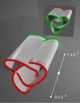
    As an alternative to the above definition of concordance using slice knots there is also a second equivalent definition. Two oriented knots K 1 {\displaystyle K_{1}} {\displaystyle K_{1}} and K 2 {\displaystyle K_{2}} {\displaystyle K_{2}} are concordant if they are the boundary of a (locally flat or smooth) cylinder C = S 1 × [ 0 , 1 ] {\displaystyle C=S^{1}\times [0,1]} {\displaystyle C=S^{1}\times [0,1]} (in the 4-dimensional space S 3 × [ 0 , 1 ] {\displaystyle S^{3}\times [0,1]} {\displaystyle S^{3}\times [0,1]}). The orientations of the two knots have to be consistent to the cylinder’s orientation, which is illustrated in the third figure. The boundary of S 3 × [ 0 , 1 ] {\displaystyle S^{3}\times [0,1]} {\displaystyle S^{3}\times [0,1]} are two S 3 {\displaystyle S^{3}} {\displaystyle S^{3}} with different orientations[8] and therefore two mirrored trefoils are shown as boundary of the cylinder. Connecting the two knots by cutting out a strip from the cylinder yields a disk, showing that for all knots the connected sum K K {\displaystyle K\sharp -K} {\displaystyle K\sharp -K} is slice. In both definitions a knot is slice if and only if it is concordant to the trivial knot.

    This can be illustrated also with the first figure at the top of this article: If a small disk at the local minimum on the bottom left is cut out then the boundary of the surface at this place is a trivial knot and the surface is a cylinder. At the other end of the cylinder we have a slice knot. If the disk (or cylinder) is smoothly embedded it can be slightly deformed to a so-called Morse position.

    This is useful because the critical points with respect to the radial function r carry geometrical meaning. At saddle points, trivial components are added or destroyed (band moves, also called fusion and fission). For slice knots any number of these band moves are possible, whereas for ribbon knots only fusions may occur and fissions are not allowed.

    In the illustration on the right the geometrical description of the concordance is rotated by 90° and the parameter r is renamed to t. This name fits well to a time interpretation of a surface ′movie′.

    4-genus

    An analogous definition as for slice knots may be done with surfaces of larger genus. The 4-genus (also called ′slice genus′) of a knot is therefore defined as the smallest genus of an embedded surface in 4-space of which the knot is the boundary. As before, we distinguish the topological and smooth 4-genus. Knots with 4-genus 0 are slice knots because a disk, the simplest surface, has genus 0. The 4-genus is always smaller or equal to the knot’s genus because this invariant is defined using Seifert surfaces which are embedded already in three-dimensional space.

    Examples for knots with different values for their topological and smooth 4-genus are listed in the following table. The Conway knot 11n34 is, as already mentioned, the first example in the knot tables for a topologically but not smoothly slice knot. Judging from the values in the table we could conclude that the smooth and the topological 4-genus always differ by 1, when they are not equal. This is not the case, however, and the difference can be arbitrarily large.[9] It is not known, though, (as of 2017), whether there are alternating knots with a difference > 1.[10]

    10 139 {\displaystyle 10_{139}} {\displaystyle 10_{139}} 10 145 {\displaystyle 10_{145}} {\displaystyle 10_{145}} 10 152 {\displaystyle 10_{152}} {\displaystyle 10_{152}} 10 154 {\displaystyle 10_{154}} {\displaystyle 10_{154}} 10 161 {\displaystyle 10_{161}} {\displaystyle 10_{161}} 11 n 34 {\displaystyle 11n34} {\displaystyle 11n34}
    4-genus (smooth) 4 2 4 3 3 1
    4-genus (top.) 3 1 3 2 2 0

    Bibliography

    • Dale Rolfsen: Knots and Links, Publish or Perish, 1976, Chapter 8.E
    • Charles Livingston: Knot theory, Carus Mathematical Monographs, 1993
    • Charles Livingston: A Survey of Classical Knot Concordance, Chapter 7 in „Handbook of Knot Theory“, Elsevier, 2005

    External links

    See also

    • Link concordance – Link equivalence relation weaker than isotopy but stronger than homotopy

    References

    1. See C. Livingston and A. H. Moore: KnotInfo: Table of Knot Invariants, https://knotinfo.math.indiana.edu/ for the notation and list of slice knots (genus-4D = 0 and genus-4D (Top.) = 0).
    2. Lisa Piccirillo: The Conway knot is not slice. Ann. of Math. 191, No. 2, p. 581–591, 2020.
    3. Andrew Casson, Cameron Gordon: Cobordism of Classical Knots, in: A. Marin, L. Guillou: A la recherche de la topologie perdue, Progress in Mathematics, Birkhäuser 1986.
    4. Ribbon diagrams for them can be found in: C. Lamm, The Search for Nonsymmetric Ribbon Knots, Exp. Math. 30, p. 349–363, 2021.
    5. The mirror variants of the knots have to be chosen in a way that the total signature is 0.
    6. Ralph Fox, John Milnor: Singularities of 2-Spheres in 4-Space and Cobordism of Knots. Osaka J. Math. 3, p. 257–267, 1966.
    7. Jacob Rasmussen: Khovanov homology and the slice genus. Inv. Math. 182, p. 419–447, 2010.
    8. For the orientation of a product see Tammo tom Dieck: Algebraic Topology, EMS Textbooks in Mathematics, 2008 (online , p. 373).
    9. P. Feller, D. McCoy: On 2-bridge knots with differing smooth and topological slice genera, Proc. Amer. Math. Soc. 144, p. 5435–5442, 2016.
    10. See the conference report Thirty Years of Floer Theory for 3-manifolds, Banff International Research Station, 2017, Problem 25, p. 12.

    This article is adapted from “Slice knot” on Wikipedia, written by its contributors, and used under CC BY-SA 4.0. Text on this page is available under the same licence. Source snapshot: Wikipedia via Kiwix, 2026-07-20.
  • Solomon’s knot

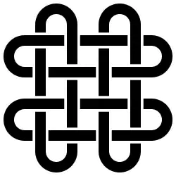
    Basic Solomon’s knot
    Solomon's knot
    Braid length 7
    Braid no. 4
    Crossing no. 4
    Hyperbolic volume 0
    Linking no. 2
    Stick no. 5
    Unknotting no. 2
    Conway notation [4]
    Thistlethwaite L4a1
    Last / Next L2a1 / L5a1
    Other
    alternating

    Solomon’s knot (Latin: sigillum Salomonis, lit.Solomon’s seal) is a traditional decorative motif used since ancient times, and found in many cultures. Despite the name, it is classified as a link, and is not a true knot according to the definitions of mathematical knot theory.

    Structure

    Solomon's knot
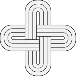
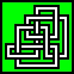
    Decorative Solomon’s knot

    The Solomon’s knot consists of two closed loops, which are doubly interlinked in an interlaced manner. If laid flat, the Solomon’s knot is seen to have four crossings where the two loops interweave under and over each other. This contrasts with two crossings in the simpler Hopf link.

    In most artistic representations, the parts of the loops that alternately cross over and under each other become the sides of a central square, while four loopings extend outward in four directions. The four extending loopings may have oval, square, or triangular endings, or may terminate with free-form shapes such as leaves, lobes, blades, wings etc.

    Occurrences

    Solomon's knot
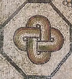
    Ancient Roman mosaic in Aquileia (Italy)

    The Solomon’s knot often occurs in ancient Roman mosaics, usually represented as two interlaced ovals.

    Sepphoris National Park, Israel, has Solomon’s Knots in stone mosaics at the site of an ancient synagogue.

    In Africa, Solomon’s knot is found on glass beadwork, textiles, and carvings of the Yoruba people. When the knot appears in this culture, it often denotes royal status; thus, it is featured on crowns, tunics, and other ceremonial objects.[1][2]

    Across the Middle East, historical Islamic sites show Solomon’s knot as part of Muslim tradition. It appears over the doorway of an early twentieth century CE mosque/madrasa in Cairo. Two versions of Solomon’s knot are included in the recently excavated Yattir Mosaic in Jordan. To the east, it is woven into an antique Central Asian prayer rug. To the west, Solomon’s knot appeared in Moorish Spain, and it shines in leaded glass windows in a late twentieth century CE mosque in the United States. The British Museum, London, England has a fourteenth-century CE Egyptian Qur’an with a Solomon’s Knot as its frontispiece.

    University of California, Los Angeles Fowler Museum of Cultural History has a large African collection that includes nineteenth and twentieth century CE Yoruba glass beadwork crowns and masks decorated with Solomon’s Knots.[1][3]

    Home of Peace Mausoleum, a Jewish Cemetery, Los Angeles, has multiple images of Solomon’s knot in stone and concrete bas reliefs sculpted 1934 CE.

    Saint Sophia’s Greek Orthodox Cathedral, “Byzantine District” of Los Angeles has an olive wood Epitaphios (bier for Christ) with Solomon’s knots carved at each corner. The Epitaphios is used in the Greek Easter services.

    Powell Library University of California, Los Angeles has ceiling beams in the Main Reading Room covered with Solomon’s Knots. Built in 1926 CE, the reading room also features a central Dome of Wisdom bordered by Solomon’s knots.[4]

    Name

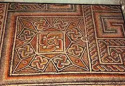
    In Latin, this configuration was sometimes known as sigillum Salomonis, meaning literally ‘seal of Solomon’. It was associated with the Biblical monarch Solomon because of his reputation for wisdom and knowledge (and in some legends, his occult powers). This phrase is usually rendered into English as “Solomon’s knot”, since “seal of Solomon” has other conflicting meanings (often referring to either a Star of David or pentagram). In the study of ancient mosaics, the Solomon’s knot is often known as a “guilloche knot” or “duplex knot”, while a Solomon’s knot in the center of a decorative configuration of four curving arcs is known as a “pelta-swastika” (where pelta is Latin for “shield”).

    Among other names currently in use are the following:

    • “Foundation Knot” applies to the interweaving or interlacing which is the basis for many elaborate Celtic designs, and is used in the United States in crochet and macramé patterns.
    • “Imbolo” describes the knot design on the textiles of the Kuba people of Congo.[5]
    • Nodo di Salomone is the Italian term for Solomon’s knot, and is used to name the Solomon’s knot mosaic found at the ruins of a synagogue at Ostia, the ancient seaport for Rome.[6]
    Solomon's knot
    Multiple Solomon’s knots in a mosaic in the Church of the Nativity (Bethlehem)
    Solomon's knot
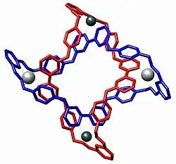
    Molecular Solomon’s knot
    Solomon's knot
    Quadruple Solomon’s knot
    Solomon's knot
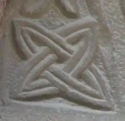
    Solomon’s knot carving in Almenno San Bartolomeo (Italy)

    See also

    References

    1. 1 2 “Solomon’s Knot – Owen W. Knight – Speculative Fiction Author”. 2020-06-09. Retrieved 2026-03-24.
    2. Lainé, Daniel, ed. (2000). African kings. Berkeley, Calif.: Ten Speed Pr. p. 63. ISBN 978-1-58008-272-3.
    3. Lainé, Daniel, ed. (2000). African kings. Berkeley, Calif.: Ten Speed Pr. ISBN 978-1-58008-272-3.
    4. “Flickr Photos”.
    5. Paulus Gerdes, Mozambican Ethnomathematics Research Centre

    6. sapere.it, Il nodo di Salomone

    Further reading

    A book-length illustrated study of Solomon’s Knot is Seeing Solomon’s Knot, With Photographs by Joel Lipton by Lois Rose Rose, Los Angeles, 2005 (official website http://www.StoneandScott.com/solomonsknot.asp Archived 2016-03-10 at the Wayback Machine).

    A few archaeological reports, art books, craft manuals, museum catalogs, auction catalogs, travel books, and religious documents which discuss or depict the Solomon’s Knot configuration are listed below:

    • Bronze Age Civilization of Central Asia, The: Recent Soviet Discoveries. Armonk, New York: M.E. Sharpe, 1981. (Early examples of Solomon’s Knot from the Gonur 1 settlement, figure 4, p. 233.)
    • Chen, Lydia. Chinese Knotting. Taiwan: Echo Publishing Company, 1981, ISBN 0-8048-1389-2. (Instructions for creating a “flat” or Solomon’s Knot, p. 58.)
    • Christie’s Catalog: The Erlenmeyer Collection of Ancient Near Eastern Stamp Seals and Amulets. London: Christie, Manson & Woods, Auction June 6, 1989. (Cruciform interlace carved stone seal, Ubaid, circa 4500 BCE, Lot 185.)
    • Fraser, Douglas and Herbert M. Cole, eds. African Art and Leadership. Madison, Milwaukee, and London: University of Wisconsin Press, 1972.
      • Cole, Ibo Art and Authority, p. 85.
      • Fraser: Symbols of Ashanti Kingship, pp. 143–144.
      • Fraser: King’s ceremonial stool, personal choices of various African leaders, p,209, p. 215, p. 283, p. 290, p. 318
      • Fraser: More attention should be paid to the significance of the Solomon’s Knot motif, p. 318.
    • Laine, Daniel. African Kings. Berkeley, Toronto: Ten Speed Press, 1991, ISBN 1-58008-272-6. (Two Nigerian chiefs, Oba Oyebade Lipede and Alake of Abeokuta, wear garments with embroidered Solomon’s Knots, p. 63.)
    • Lusini, Aldo. The Cathedral of Sienna. Sienna, Italy: 1950. (The choir stall, carved 1363 to 1425: photographs of stalls showing variations of Solomon’s Knot, plate 49, pp. 20–21.)
    • Wolpert, Stuart. “UCLA Chemists Make Molecular Rings in the Shape of King Solomon’s Knot, a Symbol of Wisdom,” News release from the University of California at Los Angeles, January 10, 2007, Newsroom.

    External links


    This article is adapted from “Solomon's knot” on Wikipedia, written by its contributors, and used under CC BY-SA 4.0. Text on this page is available under the same licence. Source snapshot: Wikipedia via Kiwix, 2026-07-20.
  • Conway knot

    Conway knot
    Conway knot
    Braid no. 3[1]
    Hyperbolic volume 11.2191
    Conway notation .−(3,2).2[2]
    Thistlethwaite 11n34
    Other
    hyperbolic, prime, slice (topological only), chiral
    Conway knot
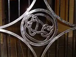
    Conway knot emblem on a closed gate at Isaac Newton Institute
    Conway knot
    Conway knot

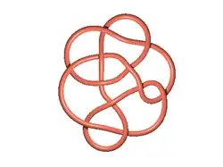
    In mathematics, specifically in knot theory, the Conway knot (or Conway’s knot) is a particular knot with 11 crossings, named after John Horton Conway.[1]

    It is related by mutation to the Kinoshita–Terasaka knot,[3] with which it shares the same Jones polynomial.[4][5] Both knots also have the property of having the same Alexander polynomial and Conway polynomial as the unknot.[6]

    The issue of the sliceness of the Conway knot was resolved in 2020 by Lisa Piccirillo, 50 years after Conway first proposed the knot.[6][7][8] Her proof made use of Rasmussen’s s-invariant, and showed that the knot is not a smoothly slice knot, though it is topologically slice (the Kinoshita–Terasaka knot is both).[9]

    References

    1. 1 2 Weisstein, Eric W. “Conway’s Knot”. mathworld.wolfram.com. Retrieved 2020-05-19.
    2. Riley, Robert (1971). “Homomorphisms of Knot Groups on Finite Groups”. Mathematics of Computation. 25 (115): 603–619. doi:10.1090/S0025-5718-1971-0295332-4.
    3. Chmutov, Sergei (2007). “Mutant Knots” (PDF). Archived (PDF) from the original on 2016-12-16.
    4. Kauffman, Louis H. “KNOTS”. homepages.math.uic.edu. Retrieved 2020-06-09.
    5. Litjens, Bart (August 16, 2011). “Knot theory and the Alexander polynomial” (PDF). esc.fnwi.uva.nl. p. 12. Archived (PDF) from the original on 2020-06-09. Retrieved 2020-06-09.
    6. 1 2 Piccirillo, Lisa (2020). “The Conway knot is not slice”. Annals of Mathematics. 191 (2): 581–591. doi:10.4007/annals.2020.191.2.5. JSTOR 10.4007/annals.2020.191.2.5.
    7. Wolfson, John. “A math problem stumped experts for 50 years. This grad student from Maine solved it in days”. Boston Globe Magazine. Retrieved 2020-08-24.
    8. Klarreich, Erica. “Graduate Student Solves Decades-Old Conway Knot Problem”. Quanta Magazine. Retrieved 2020-05-19.
    9. Klarreich, Erica. “In a Single Measure, Invariants Capture the Essence of Math Objects”. Quanta Magazine. Retrieved 2020-06-08.

    External links


    This article is adapted from “Conway knot” on Wikipedia, written by its contributors, and used under CC BY-SA 4.0. Text on this page is available under the same licence. Source snapshot: Wikipedia via Kiwix, 2026-07-20.
  • Snuggle hitch

    Snuggle hitch
    Snuggle hitch
    Category Hitch
    Origin First publication 1987
    Related Clove hitch, Ground-line hitch

    The snuggle hitch is a modification of the clove hitch, and is stronger and more secure. Owen K. Nuttall of the International Guild of Knot Tyers came up with this unique hitch, and it was first documented in the Guild’s Knotting Matters magazine issue of January, 1987.[1]
    Generally, hitches are used to attach a line to another rope or spar, pole, etc., and are usually temporary. Thus, they should be relatively easy to untie.
    [2]

    Tying

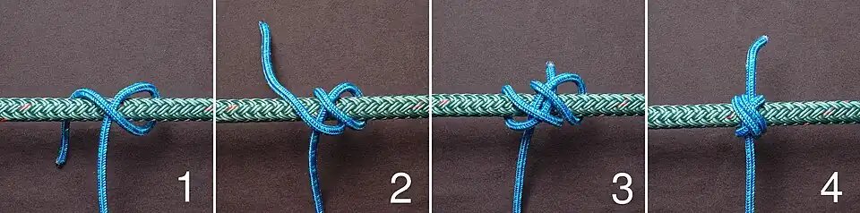
    Start by tying a clove hitch around the spar or pole. Then make an additional turn around with the working end, in the same direction as the turns forming the clove hitch. Now, tuck the working end under the standing part of the original clove hitch. Pull up tight to complete the hitch.

    • 1.  Almost a clove hitch...
      1. Almost a clove hitch…
    • 2.  Clove hitch complete...
      2. Clove hitch complete…
    • 3.  Make another turn around...
      3. Make another turn around…
    • 4.  Tuck under standing part...
      4. Tuck under standing part…
    • 5.  Pull up tight...
      5. Pull up tight…
    • 6.  Finished snuggle hitch.
      6. Finished snuggle hitch.

    See also

    References

    1. Geoffrey Budworth, The Illustrated Encyclopedia of Knots (Guilford, CT: Thalimus, 2000), 100.
    2. Joseph A. MacDonald, Handbook of Rigging (New York : McGraw Hill, 2009), 201.

    External links


    This article is adapted from “Snuggle hitch” on Wikipedia, written by its contributors, and used under CC BY-SA 4.0. Text on this page is available under the same licence. Source snapshot: Wikipedia via Kiwix, 2026-07-20.
  • Conway algebra

    In mathematics, a Conway algebra, introduced by Paweł Traczyk and Józef H. Przytycki (1988) and named after John Horton Conway, is an algebraic structure with two binary operations | and * and an infinite number of constants a1, a2,…, satisfying certain identities. Conway algebras can be used to construct invariants of links that are skein invariant.

    References

    • Traczyk, Paweł; Przytycki, Józef H. (1988), “Invariants of links of Conway type”, Kobe Journal of Mathematics, 4 (2): 115–139, ISSN 0289-9051, MR 0945888

    This article is adapted from “Conway algebra” on Wikipedia, written by its contributors, and used under CC BY-SA 4.0. Text on this page is available under the same licence. Source snapshot: Wikipedia via Kiwix, 2026-07-20.
  • Snell knot

    Snell knot
    Category Hitch
    Related Knotless knot
    Typical use Angling

    The snell knot is a hitch knot used in angling to attach a fishing line to the shank (instead of the eye) of a fishing hook. The line may still pass through the eye of the hook, but primarily fastens to the shaft. Hooks tied with a snell knot provide an even, straight-line pull to the fish. It is a very secure knot, but because it is easily tied using only the near end as the working end, it is used to attach a hook only to a leader, rather than directly to the main line.[1][2]

    Hooks can be bought pre-snelled.

    A snell knot egg hooker is used to hold a cluster of eggs or equivalent bait.[3][4]

    References

    1. “How to Tie a Snell Knot? Tips, Video & Easy Step-by-Step Guide”. 101knots.com. 25 June 2018. Retrieved 26 June 2025.
    2. “Snell Knot”. www.animatedknots.com. Retrieved 26 June 2025.
    3. Ovington, Roy (1976). Freshwater fishing. New York: Hawthorn Books. p. 60. ISBN 0-8015-2837-2.
    4. “How to Tie an Egg Loop? Steps, Variations & Video Instructions”. 101knots.com. 31 August 2018. Retrieved 26 June 2025.

    “Fishing Knots Fast”. YouTube. Retrieved 2024-11-24.


    This article is adapted from “Snell knot” on Wikipedia, written by its contributors, and used under CC BY-SA 4.0. Text on this page is available under the same licence. Source snapshot: Wikipedia via Kiwix, 2026-07-20.
  • Constrictor knot

    Constrictor knot
    Constrictor knot

    Left: constrictor knot
    Right: double constrictor knot
    Names Constrictor knot, gunner’s knot
    Category Binding
    Related Clove hitch, transom knot, strangle knot, miller’s knot, boa knot, cross constrictor knot
    Releasing Jamming
    ABoK #176, #355, #364, #430, #1188, #1189, #1249, #1250, #1251, #1252, #2052, #2097, #2489, #2560, #3441, #3700, #3853

    The constrictor knot is one of the most effective binding knots.[1][2][3][4] Simple and secure, it is a harsh knot that can be difficult or impossible to untie once tightened. It is made similarly to a clove hitch but with one end passed under the other, forming an overhand knot under a riding turn. The double constrictor knot is an even more robust variation that features two riding turns.

    History

    First called “constrictor knot” in Clifford Ashley’s 1944 work The Ashley Book of Knots, this knot likely dates back much further.[5] Although Ashley seemed to imply that he had invented the constrictor knot over 25 years before publishing The Ashley Book of Knots,[1] research indicates that he was not its only originator, but his Book of Knots does seem to be the source of subsequent knowledge and awareness of the knot.[6][7]

    Although the description is not entirely without ambiguity, the constrictor knot is thought to have appeared under the name “gunner’s knot” in the 1866 work The Book of Knots,[8][9] written under the pseudonym Tom Bowling.[a] The knot is described in relation to the clove hitch, which he illustrated and called the “builder’s knot”. He wrote, “The Gunner’s knot (of which we do not give a diagram) only differs from the builder’s knot, by the ends of the cords being simply knotted before being brought from under the loop which crosses them.”[10] But Bowling is simply an extraction and translation of the knotting work contained in the huge French Traite de L’Art de la Charpenterie, first published in 1841, which says “Le nœud de bombardier, que nous n’avons point figuré, ne differe du nœud d’artificier qu’en ce que les bouts du cordage sont croisés en nœud simple, avant de sortir de dessous la ganse qui les croise, fig.46.[11] When J. T. Burgess copied from Bowling, he changed this text to merely state “when the ends are knotted, the builder’s knot becomes the gunner’s Knot.”[12] Although a clove hitch with knotted ends is a workable binding knot,[b] Burgess was not actually describing the constrictor knot. In 1917, A. Hyatt Verrill illustrated Burgess’s clove hitch variation in Knots, Splices and Rope Work.[13]

    The constrictor knot was clearly described but not pictured as the “timmerknut” (“timber knot”) in the 1916 (2nd) edition of the Swedish book Om Knutar (“On Knots”) by Hjalmar Öhrvall.[14] Finnish scout leader Martta Ropponen presented the knot in her 1931 scouting handbook Solmukirja (“Knot Book”),[15] one of the first published works known to contain an illustration of the constrictor knot.[5] Cyrus L. Day relates that, “she had never seen it in Finland, she wrote to me in 1954, but had learned about it from a Spaniard named Raphael Gaston, who called it ‘whip knot’, and told her it was used in the mountains of Spain by muleteers and herdsmen.”[7] The Finnish name “ruoskasolmu” (“whip knot”) was a translation from Esperanto, the language Ropponen used to correspond with Gaston.[5] But even this explicit occurrence of the constrictor remains in doubt, as the name “whip knot” is not applied to the constrictor in other works, and otherwise is used for the strangle knot, tied in the ends of whip tails. Also in 1931 – and so of essentially same date as for Ropponen – James Drew presented the constrictor (as a strangle knot that can be tied in the bight) in Lester Griswold’s book, “Handicraft”; but Drew did not show it in his on book of knots later published. (As Drew knew Clifford Ashley, it is suspected that he might have learned the knot from him; Ashley does praise Handicraft in his Book of Knots.)

    Tying methods

    The method shown below is the most basic way to tie the knot around a post (that is, using a working end).[16]

    Constrictor knot
    1. Make a turn around the object and bring the working end back over the standing part.
    2. Continue around behind the object.
    3. Pass the working end over the standing part and then under the riding turn and standing part, forming an overhand knot under a riding turn.
    4. Be sure the ends emerge between the two turns as shown. Pull firmly on the ends to tighten.

    There are also at least three methods to tie the constrictor knot in the bight and slip it over the end of an object to be bound.

    Twisting method

    Using both hands when the end of the object to tie to is available:[17]

    • 1 : Both hands holding the rope, thumbs are used to form a Z with the rope
      1 : Both hands holding the rope, thumbs are used to form a Z with the rope
    • 2 : thumbs with the rope are rotated 90 degrees to cross each other forming loops
      2 : thumbs with the rope are rotated 90 degrees to cross each other forming loops
    • 3 : The resulting two loops are folded around the crossing point and held together.
      3 : The resulting two loops are folded around the crossing point and held together.
    • 4 : the resulting two loops are slipped together over the end
      4 : the resulting two loops are slipped together over the end

    If one or both of the ends are folded in between the two loops and lead in the opposite direction, the knot becomes slipped.

    Folding method

    preparing it using only one hand’s fingers:

    • 1 : a bight hanged behind ring and long finger, bottom end further inn
      1 : a bight hanged behind ring and long finger, bottom end further inn
    • 2 : ring finger end of the bight hooked by the thumb from outside and up
      2 : ring finger end of the bight hooked by the thumb from outside and up
    • 3 : long finger end of the bight hooked by the thumb from outside and down
      3 : long finger end of the bight hooked by the thumb from outside and down
    • 4 : the thumb pulls it past under the first, and rotates it by reaching out and up
      4 : the thumb pulls it past under the first, and rotates it by reaching out and up
    • 5 : long finger and thumb ends join to gather both loops around the thumb
      5 : long finger and thumb ends join to gather both loops around the thumb
    • 6 : the knot is ready to be transferred and tightened where needed
      6 : the knot is ready to be transferred and tightened where needed

    Using one hand when the end of the object to tie to is available:[18]

    • 1 : Bight turned into an underhand (overhand) loop and slipped loosely over the end of the object
      1 : Bight turned into an underhand loop and slipped loosely over the end of the object
    • 2 : The loop is grabbed from under, at the other side of crossing point, twisted half a turn (counter-)clockwise to form a number 8,
      2 : The loop is grabbed from under, at the other side of crossing point, twisted half a turn (counter-)clockwise to form a number 8,
    • 3 : Then lead over the loop crossing point and slipped a second time over the end, and finally tightened.
      3 : Then lead over the loop crossing point and slipped a second time over the end, and finally tightened.

    If the rope is to be stretched in tension, the grabbing at stage 2 may first tighten the top side rope, the bottom side rope may be pulled to tighten the knot itself, and the bottom rope side may be tightened by the knot at the next pole. If one or both of the ends are folded and led in the opposite direction before the last loop is folded over the objects end, the knot becomes slipped and therefore easier to untie: It also makes it possible to stretch either side rope tight by pulling at the slip loops.

    Variations

    Double constrictor knot

    If a stronger and even more secure knot is required an extra riding turn can be added to the basic knot to form a double constrictor knot. It is particularly useful when tying the knot with very slippery twine, especially when waxed.[2] Adding more than one extra riding turn does not add to its security and makes the knot more difficult to tighten evenly.

    Constrictor knot
    1. Make a turn around the object and bring the working end back over the standing part.
    2. Make a second turn following the same path as the first
    3. Pass the working end over the standing part, then thread it back under the standing part and both riding turns, forming an overhand knot under two riding turns.
    4. Be sure the ends emerge between the turns as shown. The double constrictor may require more careful dressing to distribute the tension throughout the knot. After working up fairly tight, pull firmly on the ends to finish.

    Slipped constrictor knot

    This variation is useful if it is known beforehand that the constrictor will need to be released. Depending on the knotting material and how tightly it is cinched, the slipped form can still be very difficult to release.

    Constrictor knot
    1. Make a turn around the object and bring the working end back over the standing part.
    2. Continue around behind the object, and then again over the standing part back to the side of the first turn.
    3. Pass a bight of the working end under the point where the first riding pass and the standing part cross to form a slip loop.
    4. Be sure the slip loop bight and both ends emerge from in between the two turns as shown.
    5. To release, tug on the working end so that the bight passes back through the knot.

    The slipped constrictor can also be tied in the bight and slipped over the object to constrict. Despite its advertised advantage (quick release), the slipped constrictor knot can also be hard to release when worked extremely tight in certain rope materials.

    Cross constrictor knot

    This variation is similar to the double constrictor knot but has the two riding turns crossing each other rather than riding along. It is unclear whether it is more secure than the double constrictor, and has the unhelpful aspect of being thicker at the bridge of the knot, with three rope diameters.

    • Step 1 of tying Cross constrictor knot: simple knot
      Step 1 of tying Cross constrictor knot: simple knot
    • Step 2 of tying Cross constrictor knot: simple knot, sides pulled to form 3 loops
      Step 2 of tying Cross constrictor knot: simple knot, sides pulled to form 3 loops
    • Step 3 of tying Cross constrictor knot: simple knot side loop folded over the middle loop
      Step 3 of tying Cross constrictor knot: simple knot side loop folded over the middle loop
    • Step 4 of tying Cross constrictor knot: the far side loop folded over the simple knot
      Step 4 of tying Cross constrictor knot: the far side loop folded over the simple knot
    • Final step of tying Cross constrictor knot: object through the 3 loops
      Final step of tying Cross constrictor knot: object through the 3 loops
    • A : turn around object at right side then at left side forming a figure-eight just like on a cleat
      A : turn around object at right side then at left side forming a figure-eight just like on a cleat
    • B : Complete the Figure-eight lashing
      B : Complete the Figure-eight lashing
    • C : Complete the overhand knot with the main line under both riding turns, entering from left
      C : Complete the overhand knot with the main line under both riding turns, entering from left
    • D : Dress
      D : Dress
    • E : Tighten
      E : Tighten

    There are two types depending on which direction the two riding turns cross. When the bottom riding turn is along the grove of the ends wrapping around each other on their way out, it gives a slightly lower knot height and may be seen as a strangle knot with an extra riding turn across.

    Usage

    Constrictor knot
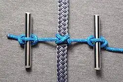
    A constrictor knot prepared for tightening using two metal rods and marlinespike hitches

    The constrictor knot is appropriate for situations where secure temporary or semi-permanent binding is needed. Made with small-stuff it is especially effective, as the binding force is concentrated over a smaller area. When tying over soft material such as the neck of a bag, take care to keep the wraps of the knot together. The constrictor knot can damage or disfigure items it is tied around.[3] To exert extreme tension on the knot without injuring the hands, one can fashion handles using marlinespike hitches made around two rods.[2]

    Constrictor knots can be used for temporarily binding the fibres of a rope (or strand ends) together while splicing, or when cutting to length and before properly whipping the ends. Constrictor knots can also be quite effective as improvised hose clamps or cable ties.[19] The knot has also been recommended as a surgical knot for ligatures in human and veterinary surgery, where it has been shown to be far superior to any of the knots commonly used for ligation.[4] Noted master-rigger Brion Toss says of the constrictor: “To know the knot is to constantly find uses for it…”[2]

    For spearguns, the constrictor knot is the usual knot used to secure modern, toggled, Dyneema, cord wishbones into the hollow, bulk-rubber loops, which are used to power the spear. Usually tied with braid, Kevlar or Dyneema cord of approximately 1.4-2mm diameter.

    Releasing

    Constrictor knot
    Cutting the riding turn

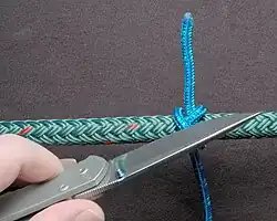
    A heavily tightened constrictor knot will likely jam. If the ends are long enough, one can sometimes untie it by pulling one end generally parallel to the bound object and a bit up away from it, and prying it into the opposite end’s part to open the knot. Tools that can be forced between parts of the knot (such as picks and marlinespikes) may help.

    If the ends have been trimmed short, or the knot is otherwise hopelessly jammed, it can be easily released by cutting the riding turn with a sharp knife. The knot will spring apart as soon as the riding turn is cut. If care is taken not to cut too deeply, the underlying wraps will protect the bound object from being damaged by the knife.[20]

    Security

    The constrictor and double constrictor are both extremely secure when tied tightly around convex objects with cord scaled for the task at hand. If binding around a not fully convex, or square-edged object, arrange the knot so the overhand knot portion is stretched across a convex portion, or a corner, with the riding turn directly atop it.[2] In situations where the object leaves gaps under the knot and there are no corners, it is possible to finish the constrictor knot off with an additional overhand knot, in the fashion of a reef knot, to help stabilize it. Those recommendations aside, constrictor knots do function best on fully convex objects.

    If the constricted object (such as a temporarily whipped rope) ends very close to where a constrictor binds it, a boa knot may prove a more stable solution.

    Notes

    1. The name “Tom Bowling” was widely associated with nautical themes, see The Adventures of Roderick Random and Charles Dibdin. The Book of Knots is most often attributed to Paul Rapsey Hodge or Frederick Chamier. For additional discussion see Ashley(1944), p. 11.
    2. A clove hitch finished with a full reef knot is still used for securing cabling in aerospace applications. See Cable lacing#Styles.

    External links

    References

    1. 1 2 Clifford W. Ashley, The Ashley Book of Knots (New York: Doubleday, 1944), 224-225.
    2. 1 2 3 4 5 Brion Toss, The Complete Rigger’s Apprentice (Camden, Maine: International Marine, 1998), 10-13.
    3. 1 2 Geoffrey Budworth, The Complete Book of Knots (London: Octopus, 1997), 136-139.
    4. 1 2 Taylor, Howard; Grogono, Alan W. (March 2014). “The constrictor knot is the best ligature”. Annals of the Royal College of Surgeons of England. 96 (2): 101–105. doi:10.1308/003588414X13814021677638. PMC 4474235. PMID 24780665.
    5. 1 2 3 Cyrus Lawrence Day, The Art of Knotting and Splicing, 4th ed. (Annapolis: Naval Institute Press, 1986), 112.
    6. Johansson, Sten (April 1983), “Letters”, Knotting Matters (3), London: International Guild of Knot Tyers: 13–14
    7. 1 2 Cyrus Lawrence Day, Quipus and Witches’ Knots (Lawrence: The University of Kansas Press, 1967), 110-111.
    8. Pieter van de Griend (1992). A Letter to Lester. Århus: Privately published. ISBN 87-983985-0-4.
    9. Pieter van de Griend (July 2007). “The Constrictor Knot Revisited”. Knot News (62). International Guild of Knot Tyers – Pacific Branch. ISSN 1554-1843.
    10. Bowling (pseudonym), Tom (1890) [1866], The Book of Knots (6th ed.), London: W. H. Allen, p. 8,
    11. Emy, Amand Rose (1870). Traite de L’Art de la Charpenterie [Treatise on the Art of Carpentry] (in French). Vol. 2 (2 ed.). Paris: Dunod. p. 589. OCLC 1016271841.
    12. Joseph Tom Burgess, Knots, Ties, and Splices (London: George Routledge & Sons, 1884), viii, 101.
    13. A. Hyatt Verrill, Knots, Splices and Rope Work, Third Revised Edition (New York: Norman W. Henly Publishing Co., 1917; 2006 Dover republication), 33-35. (second revised edition online)
    14. Hjalmar Öhrvall, Om Knutar, Second edition, (Stockholm: Albert Bonniers Förlag, 1916), 78.(Online version)
    15. Martta E. Ropponen, Kaarina Westling illustrator, Solmukirja, Suomen Partioliiton Kirjasia N:4 (Porvoo, Finland: WSOY, 1931), 58-59.
    16. “Constrictor Knot: Instrument Method”. Retrieved 4 May 2014.
    17. “Constrictor Knot: Twisting Method”. Retrieved 4 May 2014.
    18. “Constrictor Knot: Folding Method”. Retrieved 4 May 2014.
    19. “How to Tie the Impossible Knot”. HowStuffWorks. 2015-06-18. Retrieved 2022-10-12.
    20. Geoffrey Budworth, The Ultimate Encyclopedia of Knots (London: Hermes House, 1999), 159.

    This article is adapted from “Constrictor knot” on Wikipedia, written by its contributors, and used under CC BY-SA 4.0. Text on this page is available under the same licence. Source snapshot: Wikipedia via Kiwix, 2026-07-20.

  • Small knot

    Small knot
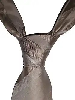
    A small knot

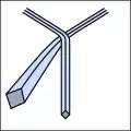
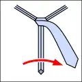
    The small knot, also known as oriental knot, Kent knot, or simple knot, is the simplest method of tying a necktie. Unlike the Four-in-hand knot and Windsor knot, the small knot is not self-releasing. The small knot is tied inside out, though this can be mitigated by giving the tie a half-twist during the tying process.

    Using the notation from The 85 Ways to Tie a Tie, the knot is tied

    • Lo Ri Co T.
    • Small knot
    • Small knot
    • Small knot

    See also

    External links


    This article is adapted from “Small knot” on Wikipedia, written by its contributors, and used under CC BY-SA 4.0. Text on this page is available under the same licence. Source snapshot: Wikipedia via Kiwix, 2026-07-20.