Category: Knots

  • Slippery hitch

    Slippery hitch
    Slippery hitch
    Category Hitch
    Related clove hitch
    Typical use To attach a line to a rod or bar.

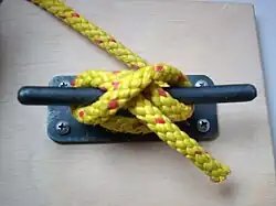
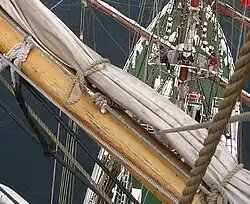
    A slippery hitch is a knot used to attach a line to a rod or bar.[1] It does not provide great strength compared to some other knots, but it can be tied relatively quickly and released very easily.[2] These characteristics mean that it is used on square-rigged ships for securing the gaskets that bind stowed sails to the yards.

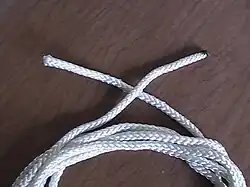
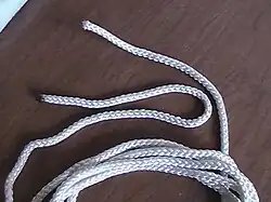
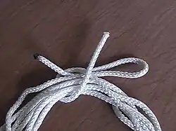
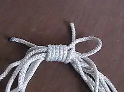
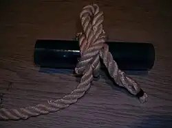
    The slippery hitch is effectively a clove hitch finished with a slipped loop. To tie one, begin as for a clove hitch, but instead of passing the end of the line through the loop in the final step, pass a bight instead, leaving the end on the original side. Pulling on this end will release the hitch. If tied in a gasket, this will quickly release the sail.

    Slippery hitch
    A slippery hitch – a clove hitch with a loop in the end.

    See also

    References

    1. McEwen, T. (2006). Boater’s Pocket Reference: Your Comprehensive Resource for Boats and Boating. Anchor Cove Pub. p. 387. ISBN 978-0-9774052-0-6. Retrieved 14 November 2024.
    2. Cruising World. p. 2-PA128. ISSN 0098-3519. Retrieved 14 November 2024.

    This article is adapted from “Slippery hitch” on Wikipedia, written by its contributors, and used under CC BY-SA 4.0. Text on this page is available under the same licence. Source snapshot: Wikipedia via Kiwix, 2026-07-20.

  • Common whipping

    Common whipping
    Names Common whipping, Plain whipping, Ordinary whipping, Wolf whipping
    Category Whipping
    ABoK #3442

    The common whipping is the simplest type of whipping knot, a series of knots intended to stop a rope from unravelling. As it can slip off the rope easily, the common whipping should not be used for rope ends that will be handled. This whipping knot is also called ‘wolf’ whipping in some parts of the world. The ‘Hangman’s knot‘ is a variation of this whipping knot.

    The benefit of a common whipping is that no tools are necessary and the rope does not need to be unlaid. The problem is that it will slide off the end of the rope with little provocation. Other whippings avoid this by interleaving the whipping with the strands of the rope and creating friction with the strands to avoid slipping.

    Normally a natural fibre rope is whipped with twine. The size of the rope dictates the size of the twine. Any twine can be used, but tarred two strand hemp (marline) is preferred. Artificial-fibre ropes should have their ends fused by heat rather than whipped to prevent unravelling.

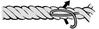
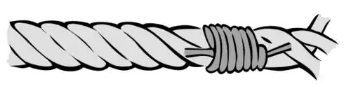
    Common, plain or ordinary whipping is tied by laying a loop along the rope and then making a series of turns over it. The working end is finally stuck through this loop and the end hauled back out of sight. Both ends are then trimmed short.

    Process

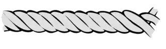
    rope without whipping

    The rope should be whipped a short distance (One and a half times the diameter) from its end.

    whipping step 1

    Lay the head of the twine along the rope, make a bight back along the rope

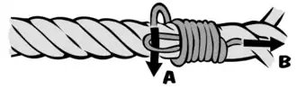
    whipping step 2

    Begin wrapping the twine around the rope and bight of twine securely.

    Wrap until the whipping is one and a half times wider than the rope is thick

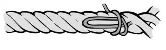
    whipping step 3

    Slip the working end of the twine through the bight.
    Carefully pull on the standing end of the twine until the bight and working end are pulled under the whipping (Note: It is normally necessary to maintain tension on the working end to prevent the bight from being dragged completely through and so destroying the whipping)

    whipping - finished

    Cut the twine flush with the edges of the whipping and the rope end not less than half its width from the whipping to give the rope end a finished look

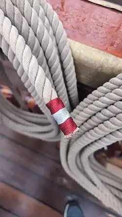
    A series of common whipping knots used to make the flag of Peru on the BAP Unión
    A series of common whipping knots used to make the flag of Peru on the BAP Unión

    See also

    References

    1. Ashley, Clifford W. (1944). The Ashley Book of Knots, p.546. Doubleday. ISBN 0-385-04025-3.

    Further reading


    This article is adapted from “Common whipping” on Wikipedia, written by its contributors, and used under CC BY-SA 4.0. Text on this page is available under the same licence. Source snapshot: Wikipedia via Kiwix, 2026-07-20.

  • Slippery eight loop

    Slippery eight loop
    Slippery eight loop
    Category Loop
    Origin Dave Poston
    Releasing Non-jamming

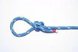
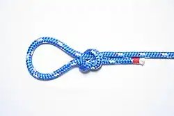
    The slippery eight loop is an adjustable loop knot discovered by Dave Poston in 2002.

    Information

    The slippery eight loop is known — despite the name — to have an extraordinary ability to not slip and it is extremely secure when the legs are at less than a 90-degree angle. The man who created this knot, Dave Poston, requests that the name of the knot include “HFP” in order to honor his father, who originally introduced him to knots. So the whole name of the knot would be the “HFP Slippery 8 Loop.”[1]

    Instructions

    The instructions on how to create a slippery eight loop is as follows:

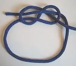
    1. Begin by creating a figure eight knot with one end long enough to be looped through it again
    2. Make sure that the figure eight loop is not tight, but rather quite loose with obvious gaps
    3. Bring the long, working end to the top of the knot
    4. Pass the working end behind the standing line in the knot and feed the end through the Eight
    5. After the working end has been threaded through the knot, pull the knot tight
    6. Adjust the size of the loop by alternately pulling the different ends or one side of the loop

    See also

    References

    1. “HFP Slippery 8 Loop”. Notable Knot Index. Retrieved 11 May 2013.

    External links


    This article is adapted from “Slippery eight loop” on Wikipedia, written by its contributors, and used under CC BY-SA 4.0. Text on this page is available under the same licence. Source snapshot: Wikipedia via Kiwix, 2026-07-20.

  • Coiling

    Coiling
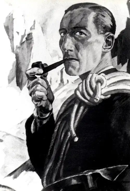
    Self-portrait of Erwin Merlet with a mountaineer’s coil slung over his shoulder and the Sella Towers in the background.

    A coiling or coil is a curve, helix, or spiral used for storing rope or cable in compact and reliable yet easily attainable form. They are often discussed with knots.

    Rope are often coiled and hung up in lofts for storage. They are also hung over stakes in farm wagons and on hooks in moving vans, fire apparatus and linesmen’s repair trucks. For such active storage coils must be well made.

    Mountaineer’s coil

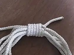
    The mountaineer’s coil (also alpine coil, climber’s coil, lap coil, or standing coil[2]) is a traditional method used by climbers to store and transport a climbing rope.[3] This older style coil is noted as being more prone to twists and tangles than the butterfly coil, and care must be taken upon uncoiling to avoid these problems.[2][3][4]

    Tying method

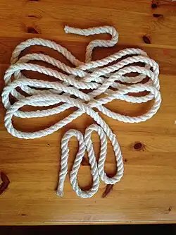
    Begin by taking hold of the rope in one hand with its end facing you. Coil the rope in arm’s length sections with your free hand (extending it away from the other as far as it will reach to ensure each segment is of equal length as it is gathered). Alternate tucking the new gather in front and behind the previous coil to avoid putting a half-turn in the rope with each coil.[4]

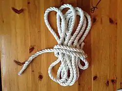
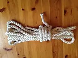
    When the last segment is reached form a short bight atop the gathered rope with its standing end. Grasp the working end and pass it over the bight and back through the center of the coiled rope in a round turn several times, making each new wrap closer to the bight until only a short tail remains. Pass this tail through the bight then grasp the standing end and pull it away from the bight until it is cinched tight around the working end.[4][5]

    For added security, ensure both ends are sufficiently long to tie them into a reef knot.[3]

    Forming the coil
    Coiling
    Coil the rope until its ends are reached
    Coiling
    Make a bight in one end (the standing end)
    Coiling
    Wrap the opposite end (the working end) around the coil in a round turn
    Coiling
    Make several additional round turns then insert the working end through the bight
    Coiling
    Pull the standing end to tighten the bight and complete the knot

    Butterfly coil

    Coiling
    Tying the Butterfly coil, 1-folding or faking-down
    Coiling
    Tying the Butterfly coil, 2-wrapping
    Coiling
    Tying the Butterfly coil, 3-finished

    The butterfly coil (also known as a backpacker’s coil) is a method used by climbers for storing and transporting a climbing rope. Slinging the coiled rope over the shoulders and tying it in place for carrying earns the technique its alternative name.[6]

    Unlike the alpine coil it cannot be attached to a harness for climbing, and thus is useful only for transporting a rope to and from where it must be used.

    The method is also useful for much smaller items such as for keeping earphone cables from tangling.

    Tying method

    Depending on the thickness and length, one can use palms of hands stretched out to the sides (crossing over the neck), two knees, passive side palm and elbow, or two fingers of the passive hand. The following is for the extra long climbing rope.

    Start with both rope ends in one hand. Pull 1.5–2 arm lengths of the pair through and let their ends hang free. Begin coiling the balance of both strands one arm length at a time, alternating the gathers in the opposite hand into two separate “lobes” (or wings) draping on either side.[7]

    With 1.5–2 arm lengths remaining secure the coil by wrapping both strands twice round both lobes approximately 1–1.5′ down, then pass a short bight above the wraps and through the coil. Pass both free ends over the top of the coil and through the bight to cinch it tight.

    Attach the rope for transport by placing the coil atop one’s back, with one free end passing over each shoulder. Pass the ends back under the armpits, cross them over the coil, then bring them forward again, securing in front with a square knot.

    An alternate method draws the doubled rope over the shoulders instead of in front of the climber.

    Over/under cable coiling

    Over/under cable coiling refers to a method of storing cables that preserves the capacitance and common-mode rejection ratio built in by the manufacturer with a twist in the cable, and the shielding that encases the twisted pairs within. It allows the cable to lie flat when uncoiled, and makes for easier and faster work.

    The “over/under” name refers to the practice of twisting the cable in one direction to make the first coil, and un-twisting it to make the next, and repeating this until all the cable is neatly coiled. Care needs to be taken to keep each end on its proper side of the roll when uncoiling otherwise a knot will appear with every other loop. Connecting the ends on the outside of the loops, or tying them in that position, ensures that the ends don’t pass through the loops in storage so there are no knots when the cable is laid out.[8]

    There are a number of informal terms in common circulation including “over/under wrapping”, “countercoiling”, and “flip-coiling”.[9]

    Straight coiling

    Straight coiling, or the practice of coiling a cable in the same direction coil after coil, has the similar result to coiling cable on a spool. If the cable comes off the spool the same way it goes on, the internal ‘lay’ is preserved, and the cable isn’t damaged or twisted internally. If a cable is straight coiled and then pulled from the coil, it has the effect as coiling cable on a spool and then pulling the cable off the top of the spool, imparting a twist in the cable with every coil that is removed. To make it lie flat, the twist will need to be removed. The advantages of straight coiling cable are that it will not produce knots when uncoiling and is easily taught and therefore can be accomplished easily by assistants.

    See also

    • Sheepshank, also known as shank knot – Type of knot
    • Chain sinnet – Series of knots for shortening a cable

    References

    1. Ashley, Clifford W. (1944). The Ashley Book of Knots, p.513. Doubleday. ISBN 0-385-04025-3.
    2. 1 2 Soles, Clyde (2004), The Outdoor Knot Book, Seattle: The Mountaineers Books, pp. 67–69, ISBN 978-0-89886-962-0
    3. 1 2 3 Eng, Ronald C., ed. (2010). Mountaineering – Freedom of the Hills (8th ed.). Seattle: The Mountaineers Books. p. 137.
    4. 1 2 3 “Coiling Unattached Rope”. Grog LLC. Retrieved 2012-03-13.
    5. “Coil Your Rope for Imminent Use”. ITS Tactical. 2009-12-21. Retrieved 2012-03-13.
    6. “Rock Seconding School Student Manual”. July 2006. Archived from the original on 2007-03-13. Retrieved 2006-10-19.
    7. Bluewater Beta: The Backpacker’s Coil
    8. Fielden, John (February 6, 2010). Roll Sound!. My Planet Marketing. p. 36. ISBN 9781450549837.
    9. “Flip-coiling”.

    External links


    This article is adapted from “Coiling” on Wikipedia, written by its contributors, and used under CC BY-SA 4.0. Text on this page is available under the same licence. Source snapshot: Wikipedia via Kiwix, 2026-07-20.

  • Slip knot

    Slip knot
    Slip knot

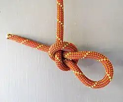
    A slip knot tied in a kernmantle rope
    Names Slip knot, Slipped overhand knot
    Category Stopper
    Related overhand knot, noose knot, running knot
    Releasing Non-jamming
    Typical use temporary stopper knot, knitting, animal snares
    ABoK 529[1]

    The slip knot is a stopper knot which is easily undone by pulling the tail (working end). The slip knot is related to the running knot, which will release when the standing end is pulled. Both knots are identical and are composed of a slipped overhand knot, where a bight allows the knot to be released by pulling on an end; the working end for a slip knot, and the standing end for a running knot. The slip knot is used as a starting point for crochet and knitting.

    The slip knot is a stopper knot that may be spilled or slipped instantly by pulling on the end to withdraw a loop. There is but one knot entitled to the name; any others having a similar feature are merely “slipped” knots. — The Ashley Book of Knots[1]

    Standard creation

    Slip knot
    Slip knot
    Slip knot
    Noose
    Slip knot
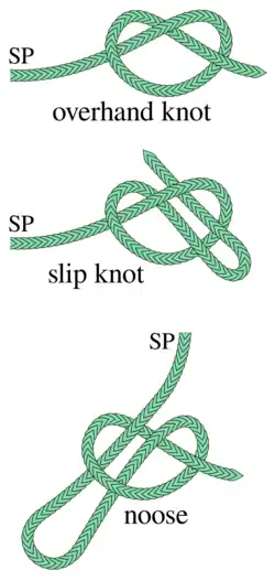
    overhand knot, slip knot, noose

    The slip knot is closely related to the overhand knot, the difference between the two being in the treatment of the end. In the former the end is doubled before it is finally tucked. To untie, all that is required is a smart pull on the end of the rope, which withdraws the loop and causes the knot to spill instantly. A slip knot may be tied in the bight as readily as in the end, but the load must be on the standing part of the knot only. It is used wherever the necessity to cast off suddenly may arise.

    The slip knot is formed by first creating a loop in the shape of a “p”. Place a hand or hook through the loophole and grab a bight on the working end. Draw this bight through the first loop. Seat the knot and pull the bight until a small loop is created.

    See also

    References

    1. 1 2 3 Ashley, Clifford W. (1993) [1944]. The Ashley Book of Knots. New York: Doubleday. pp. 87, 14. ISBN 0-385-04025-3.

    External links


    This article is adapted from “Slip knot” on Wikipedia, written by its contributors, and used under CC BY-SA 4.0. Text on this page is available under the same licence. Source snapshot: Wikipedia via Kiwix, 2026-07-20.

  • Slice genus

    In mathematics, the slice genus of a smooth knot K in S3 (sometimes called its Murasugi genus or 4-ball genus) is the least integer g such that K is the boundary of a connected, compact, orientable 2-manifold S of genus g properly embedded in the 4-ball D4 bounded by S3.

    More precisely, if S is required to be smoothly embedded, then this integer g is the smooth slice genus of K and is often denoted gs(K) or g4(K), whereas if S is required only to be topologically locally flatly embedded then g is the topologically locally flat slice genus of K. (There is no point considering g if S is required only to be a topological embedding, since the cone on K is a 2-disk with genus 0.) There can be an arbitrarily great difference between the smooth and the topologically locally flat slice genus of a knot; a theorem of Michael Freedman says that if the Alexander polynomial of K is 1, then the topologically locally flat slice genus of K is 0, but it can be proved in many ways (originally with gauge theory) that for every g there exist knots K such that the Alexander polynomial of K is 1 while the genus and the smooth slice genus of K both equal g.

    The (smooth) slice genus of a knot K is bounded below by a quantity involving the ThurstonBennequin invariant of K:

    g s ( K ) ( T B ( K ) + 1 ) / 2. {\displaystyle g_{s}(K)\geq ({\rm {TB}}(K)+1)/2.\,} {\displaystyle g_{s}(K)\geq ({\rm {TB}}(K)+1)/2.\,}

    The (smooth) slice genus is zero if and only if the knot is concordant to the unknot.

    See also

    Further reading

    • Livingston Charles, A survey of classical knot concordance, in: Handbook of knot theory, pp 319347, Elsevier, Amsterdam, 2005. MR 2179265 ISBN 0-444-51452-X


    This article is adapted from “Slice genus” on Wikipedia, written by its contributors, and used under CC BY-SA 4.0. Text on this page is available under the same licence. Source snapshot: Wikipedia via Kiwix, 2026-07-20.

  • Cleat hitch

    Cleat hitch
    Cleat hitch
    Names Cleat hitch, cleat knot, cleat tie
    Category Hitch
    Origin Nautical
    Releasing Non-jamming[1]
    ABoK #1615
    Instructions

    The cleat hitch is a knot for securely attaching a rope to a cleat.

    Tying

    The hitch begins with a dead turn around the cleat then continues forming an “8”. The hitch is finished with an inverted half hitch.

    • A dead turn
      A dead turn
    • We cross by making an eight
      We cross by making an eight
    • Prepare the reverse half hitch
      Prepare the reverse half hitch
    • The finished knot
      The finished knot

    See also

    Notes

    Bibliography

    • Ashley, Clifford W. (1993) [1944], The Ashley Book of Knots, New York: Doubleday, p. Dust jacket, ISBN 0-385-04025-3 p.286
    • Compton, Nic (2013), The Knot Bible, The complete guide to knots and their uses, London: Adlard Coles Nautical, ISBN 978-1-4081-5476-2 p.66
    • Soles, Clyde (2011), Backpacker magazine’s outdoor knots : the knots you need to know, Morris Book Publishing, LLC, ISBN 978-0-7627-5651-3 p.72

    References

    External links


    This article is adapted from “Cleat hitch” on Wikipedia, written by its contributors, and used under CC BY-SA 4.0. Text on this page is available under the same licence. Source snapshot: Wikipedia via Kiwix, 2026-07-20.

  • Clasper (mathematics)

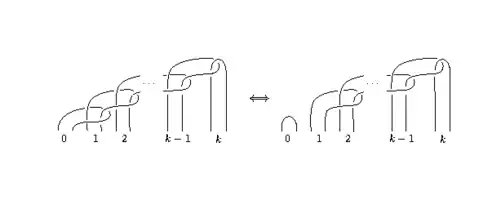
    In the mathematical field of low-dimensional topology, a clasper is a surface (with extra structure) in a 3-manifold on which surgery can be performed.

    Motivation

    Beginning with the Jones polynomial, infinitely many new invariants of knots, links, and 3-manifolds were found during the 1980s. The study of these new `quantum’ invariants expanded rapidly into a sub-discipline of low-dimensional topology called quantum topology. A quantum invariant is typically constructed from two ingredients: a formal sum of Jacobi diagrams (which carry a Lie algebra structure), and a representation of a ribbon Hopf algebra such as a quantum group. It is not clear a-priori why either of these ingredients should have anything to do with low-dimensional topology. Thus one of the main problems in quantum topology has been to interpret quantum invariants topologically.

    The theory of claspers comes to provide such an interpretation. A clasper, like a framed link, is an embedded topological object in a 3-manifold on which one can perform surgery. In fact, clasper calculus can be thought of as a variant of Kirby calculus on which only certain specific types of framed links are allowed. Claspers may also be interpreted algebraically, as a diagram calculus for the braided strict monoidal category Cob of oriented connected surfaces with connected boundary. Additionally, most crucially, claspers may be roughly viewed as a topological realization of Jacobi diagrams, which are purely combinatorial objects. This explains the Lie algebra structure of the graded vector space of Jacobi diagrams in terms of the Hopf algebra structure of Cob.

    Definition

    A clasper G = A B {\displaystyle G=\mathbf {A} \cup \mathbf {B} } {\displaystyle G=\mathbf {A} \cup \mathbf {B} } is a compact surface embedded in the interior of a 3-manifold M {\displaystyle M} {\displaystyle M} equipped with a decomposition into two subsurfaces A {\displaystyle \mathbf {A} } {\displaystyle \mathbf {A} } and B {\displaystyle \mathbf {B} } {\displaystyle \mathbf {B} }, whose connected components are called the constituents and the edges of G {\displaystyle G} {\displaystyle G} correspondingly. Each edge of G {\displaystyle G} {\displaystyle G} is a band joining two constituents to one another, or joining one constituent to itself. There are four types of constituents: leaves, disk-leaves, nodes, and boxes.

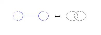
    Clasper surgery is most easily defined (after elimination of nodes, boxes, and disk-leaves as described below) as surgery along a link associated to the clasper by replacing each leaf with its core, and replacing each edge by a right Hopf link.

    Clasper (mathematics)

    Clasper calculus

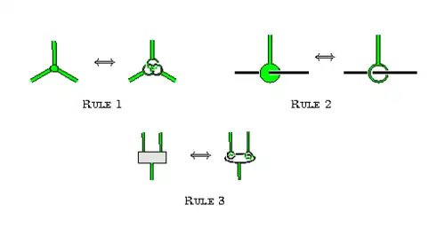
    The following are the graphical conventions used when drawing claspers (and may be viewed as a definition for boxes, nodes, and disk-leaves):

    Clasper (mathematics)
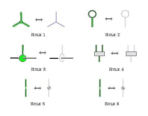
    Replacing nodes, disk-leaves, and boxes with leaves
    Clasper (mathematics)
    Convensions drawing claspers

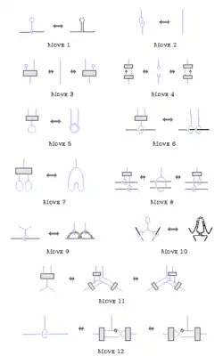
    Habiro found 12 moves which relate claspers along which surgery gives the same result. These moves form the core of clasper calculus, and give considerable power to the theory as a theorem-proving tool.

    Clasper (mathematics)
    Habiro’s twelve moves.

    Cn-equivalence

    Two knots, links, or 3-manifolds are said to be C n {\displaystyle C_{n}} {\displaystyle C_{n}}-equivalent if they are related by C n {\displaystyle C_{n}} {\displaystyle C_{n}}-moves, which are the local moves induced by surgeries on a simple tree claspers without boxes or disk-leaves and with n {\displaystyle n} {\displaystyle n} leaves.

    Clasper (mathematics)
    A C n {\displaystyle C_{n}} {\displaystyle C_{n}}-move.

    For a link L M {\displaystyle L\subset M} {\displaystyle L\subset M}, a C 1 {\displaystyle C_{1}} {\displaystyle C_{1}}-move is a crossing change. A C 2 {\displaystyle C_{2}} {\displaystyle C_{2}}-move is a Delta move. Most applications of claspers use only C n {\displaystyle C_{n}} {\displaystyle C_{n}}-moves.

    Main results

    For two knots K {\displaystyle K} {\displaystyle K} and K {\displaystyle K^{\prime }} {\displaystyle K^{\prime }} and a non-negative integer k {\displaystyle k} {\displaystyle k}, the following conditions are equivalent:

    1. K {\displaystyle K} {\displaystyle K} and K {\displaystyle K^{\prime }} {\displaystyle K^{\prime }} are not distinguished by any invariant of type k {\displaystyle k} {\displaystyle k}.
    2. K {\displaystyle K} {\displaystyle K} and K {\displaystyle K^{\prime }} {\displaystyle K^{\prime }} are C k {\displaystyle C_{k}} {\displaystyle C_{k}}-equivalent.

    The corresponding statement is false for links.

    Further reading

    • S. Garoufalidis, M. Goussarov, and M. Polyak, Calculus of clovers and finite-type invariants of 3-manifolds, Geom. and Topol., vol. 5 (2001), 75108.
    • M.N. Goussarov, Variations of knotted graphs. The geometric technique of n-equivalence (Russian) Algebra i Analiz 12(4) (2000), 79–125; translation in St. Petersburg Math. J. 12(4) (2001) 569–604.
    • M.N. Goussarov, Finite type invariants and n-equivalence of 3-manifolds C. R. Acad. Sci. Paris Ser. I Math. 329(6) (1999), 517–522.
    • K. Habiro, Claspers and the Vassiliav skein module, PhD thesis, University of Tokyo (1997).
    • K. Habiro, Claspers and finite type invariants of links, Geom. and Topol., vol. 4 (2000), 183.
    • S. Matveev, Generalized surgeries of three-dimensional manifolds and representations of homology spheres, Mat. Zametki, 42 (1987) no. 2, 268–278.


    This article is adapted from “Clasper (mathematics)” on Wikipedia, written by its contributors, and used under CC BY-SA 4.0. Text on this page is available under the same licence. Source snapshot: Wikipedia via Kiwix, 2026-07-20.

  • Skein relation

    Skein relations are a mathematical tool used to study knots. A central question in the mathematical theory of knots is whether two knot diagrams represent the same knot. One way to answer the question is using knot polynomials, which are invariants of the knot. If two diagrams have different polynomials, they represent different knots. However, the converse is not true.

    Skein relations are often used to give a simple definition of knot polynomials. A skein relation gives a linear relation between the values of a knot polynomial on a collection of three links which differ from each other only in a small region. For some knot polynomials, such as the Conway, Alexander, and Jones polynomials, the relevant skein relations are sufficient to calculate the polynomial recursively.

    Definition

    A skein relationship requires three link diagrams that are identical except at one crossing. The three diagrams must exhibit the three possibilities that could occur for the two line segments at that crossing, one of the lines could pass under, the same line could be over or the two lines might not cross at all. Link diagrams must be considered because a single skein change can alter a diagram from representing a knot to one representing a link and vice versa. Depending on the knot polynomial in question, the links (or tangles) appearing in a skein relation may be oriented or unoriented.

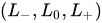
    The three diagrams are labelled as follows. Turn the three link diagram so the directions at the crossing in question are both roughly northward. One diagram will have northwest over northeast, it is labelled L. Another will have northeast over northwest, it’s L+. The remaining diagram is lacking that crossing and is labelled L0.
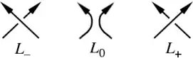
    Skein relation

    (The labelling is independent of direction insofar as it remains the same if all directions are reversed. Thus polynomials on undirected knots are unambiguously defined by this method. However, the directions on links are a vital detail to retain as one recurses through a polynomial calculation.)

    It is also sensible to think in a generative sense, by taking an existing link diagram and “patching” it to make the other twojust so long as the patches are applied with compatible directions.

    To recursively define a knot (link) polynomial, a function F is fixed and for any triple of diagrams and their polynomials labelled as above,
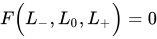
    F ( L , L 0 , L + ) = 0 {\displaystyle F{\Big (}L_{-},L_{0},L_{+}{\Big )}=0} {\displaystyle F{\Big (}L_{-},L_{0},L_{+}{\Big )}=0}

    or more pedantically

    F ( L ( x ) , L 0 ( x ) , L + ( x ) , x ) = 0 {\displaystyle F{\Big (}L_{-}(x),L_{0}(x),L_{+}(x),x{\Big )}=0} {\displaystyle F{\Big (}L_{-}(x),L_{0}(x),L_{+}(x),x{\Big )}=0} for all x {\displaystyle x} {\displaystyle x}

    (Finding an F which produces polynomials independent of the sequences of crossings used in a recursion is no trivial exercise.)

    More formally, a skein relation can be thought of as defining the kernel of a quotient map from the planar algebra of tangles. Such a map corresponds to a knot polynomial if all closed diagrams are taken to some (polynomial) multiple of the image of the empty diagram.

    Example

    Sometime in the early 1960s, Conway showed how to compute the Alexander polynomial using skein relations. As it is recursive, it is not quite so direct as Alexander’s original matrix method; on the other hand, parts of the work done for one knot will apply to others. In particular, the network of diagrams is the same for all skein-related polynomials.

    Let function P from link diagrams to Laurent series in x {\displaystyle {\sqrt {x}}} {\displaystyle {\sqrt {x}}} be
    such that P ( u n k n o t ) = 1 {\displaystyle P({\rm {unknot}})=1} {\displaystyle P({\rm {unknot}})=1} and a triple of skein-relation diagrams ( L , L 0 , L + ) {\displaystyle (L_{-},L_{0},L_{+})} {\displaystyle (L_{-},L_{0},L_{+})} satisfies the equation
    P ( L ) = ( x 1 / 2 x 1 / 2 ) P ( L 0 ) + P ( L + ) {\displaystyle P(L_{-})=(x^{-1/2}-x^{1/2})P(L_{0})+P(L_{+})} {\displaystyle P(L_{-})=(x^{-1/2}-x^{1/2})P(L_{0})+P(L_{+})}

    Then P maps a knot to one of its Alexander polynomials.

    In this example, we calculate the Alexander polynomial of the cinquefoil knot (Skein relation), the alternating knot with five crossings in its minimal diagram. At each stage we exhibit a relationship involving a more complex link and two simpler diagrams. Note that the more complex link is on the right in each step below except the last. For convenience, let A = x−1/2−x1/2.

    To begin, we create two new diagrams by patching one of the cinquefoil’s crossings (highlighted in yellow) so

    P(Skein relation) = A × P(Skein relation) + P(Skein relation)

    The second diagram is actually a trefoil; the first diagram is two unknots with four crossings. Patching the latter

    P(Skein relation) = A × P(Skein relation) + P(Skein relation)

    gives, again, a trefoil, and two unknots with two crossings (the Hopf link ). Patching the trefoil

    P(Skein relation) = A × P(Skein relation) + P(Skein relation)

    gives the unknot and, again, the Hopf link. Patching the Hopf link

    P(Skein relation) = A × P(Skein relation) + P(Skein relation)

    gives a link with 0 crossings (unlink) and an unknot. The unlink takes a bit of sneakiness:

    P(Skein relation) = A × P(Skein relation) + P(Skein relation)

    Computations

    We now have enough relations to compute the polynomials of all the links we’ve encountered, and can use the above equations in reverse order to work up to the cinquefoil knot itself. The calculation is described in the table below, where ? denotes the unknown quantity we are solving for in each relation:

    knot name diagrams P (diagram)
    skein equation ? P in full
    unknot Skein relation Skein relation Skein relation Skein relation defined as 1 x→1
    unlink Skein relation Skein relation 1=A?+1 0 x→0
    Hopf link Skein relation Skein relation Skein relation 0=A1+? -A x→x1/2-x−1/2
    trefoil Skein relation Skein relation Skein relation 1=A(-A)+? 1+A2 x→x−1-1+x
    4 crossing link Skein relation Skein relation -A=A(1+A2)+? -A(2+A2) x→-x−3/2+x−1/2-x1/2+x3/2
    cinquefoil Skein relation 1+A2=A(-A(2+A2))+? 1+3A2+A4 x→x−2-x−1+1-x+x2

    Thus the Alexander polynomial for a cinquefoil is P(x) = x−2 -x−1 +1 -x +x2.

    Etymology

    In knot theory, the term skein appears to have been coined by John Conway around 1979, and refers to the unit of measure of yarn in the textiles industry.

    Sources


    This article is adapted from “Skein relation” on Wikipedia, written by its contributors, and used under CC BY-SA 4.0. Text on this page is available under the same licence. Source snapshot: Wikipedia via Kiwix, 2026-07-20.
  • Circuit topology

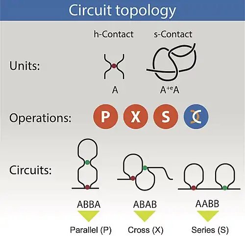
    Circuit topology relations in a chain with two binary contacts.
    Circuit topology relations in a chain with two binary contacts.

    The circuit topology of a folded linear polymer is the arrangement of its intra-molecular contacts. Examples of linear polymers with intra-molecular contacts are nucleic acids and proteins. Proteins fold via the formation of contacts of various natures, including hydrogen bonds, disulfide bonds, and beta-beta interactions.[1] RNA molecules fold by forming hydrogen bonds between nucleotides, forming nested or non-nested structures. Contacts in the genome are established via protein bridges including CTCF and cohesins and are measured by technologies including Hi-C.[2] Circuit topology categorizes the topological arrangement of these physical contacts, that are referred to as hard contacts (or h-contacts). Furthermore, chains can fold via knotting (or the formation of “soft” contacts (s-contacts)). Circuit topology uses a similar language to categorize both “soft” and “hard” contacts, and provides a full description of a folded linear chain. In this framework, a “circuit” refers to a segment of the chain where each contact site within the segment forms connections with other contact sites within the same segment, and thus is not left unpaired. A folded chain can thus be studied based on its constituting circuits.

    A simple example of a folded chain is a chain with two hard contacts. For a chain with two binary contacts, three arrangements are available: parallel (P), series (S), and crossed (X). For a chain with n contacts, the topology can be described by an n by n matrix in which each element illustrates the relation between a pair of contacts and may take one of the three states, P, S and X. Multivalent contacts can also be categorised in full or via decomposition into several binary contacts. Similarly, circuit topology allows for the classification of the pairwise arrangements of chain crossings and tangles, thus providing a complete 3D description of folded chains. Furthermore, one can apply circuit topology operations to soft and hard contacts to generate complex folds, using a bottom-up engineering approach.

    Both knot theory and circuit topology aim to describe chain entanglement, making it important to understand their relationship. Knot theory considers any entangled chain as a connected sum of prime knots, which are themselves undecomposable. Circuit topology splits any entangled chains (including prime knots) into basic structural units called soft contacts, and lists simple rules on how soft contacts can be put together.[3][4] An advantage of circuit topology is that it can be applied to open linear chains with intra-chain interactions, so-called hard contacts.[5] This enabled topological analysis of proteins and genomes, which are often described as unknot in knot theory.[6][7] Finally, circuit topology enables studying interactions between hard contacts and entanglements and can identify slip knots, while knot theory typically overlooks hard contacts and split knots. Thus, circuit topology serves as a complementary approach to knot theory.

    Circuit topology has implications for folding kinetics and molecular evolution and has been applied to engineer polymers including molecular origami.[8][9] Circuit topology along with contact order and size are determinants of the folding rate of linear polymers.[10] It has also been applied to quantify the conformational organisation of intrinsically disordered proteins.[11][12][13] In protein structure prediction, coarse-grained generative approaches recover global topological features of protein folds and enable rapid contact map prediction.[14] Circuit topology can be applied to characterise the topology of multi-chain systems as well, including biomolecular condensates and aggregates.[15][16] For example, it has been used to characterise coil–globule transitions and aggregation in polymers, revealing multichain topological motifs during collective structural transitions.[17] In addition, circuit topology has been applied to classify conformational substates in amyloid polypeptides, providing insight into aggregation mechanisms and their modulation by small molecules.[18] Finally, the topology approach can also be used for medical applications including disease analysis,[19] and drug response predictions.[20][21]

    See also

    • Topology (chemistry)

    Further reading

    References

    1. Mashaghi, Alireza; van Wijk, Roeland J.; Tans, Sander J. (2014). “Circuit Topology of Proteins and Nucleic Acids”. Structure. 22 (9): 1227–1237. doi:10.1016/j.str.2014.06.015. PMID 25126961.
    2. Scalvini, Barbara; Schiessel, Helmut; Golovnev, Anatoly; Mashaghi, Alireza (March 2022). “Circuit topology analysis of cellular genome reveals signature motifs, conformational heterogeneity, and scaling”. iScience. 25 (3) 103866. Bibcode:2022iSci…25j3866S. doi:10.1016/j.isci.2022.103866. PMC 8861635. PMID 35243229.
    3. Golovnev, Anatoly; Mashaghi, Alireza (7 December 2021). “Circuit Topology for Bottom-Up Engineering of Molecular Knots”. Symmetry. 13 (12): 2353. arXiv:2106.03925. Bibcode:2021Symm…13.2353G. doi:10.3390/sym13122353.
    4. Flapan, Erica; Mashaghi, Alireza; Wong, Helen (1 June 2023). “A tile model of circuit topology for self-entangled biopolymers”. Scientific Reports. 13 (1): 8889. Bibcode:2023NatSR..13.8889F. doi:10.1038/s41598-023-35771-8. PMC 10235088. PMID 37264056. S2CID 259022790.
    5. Golovnev, Anatoly; Mashaghi, Alireza (September 2020). “Generalized Circuit Topology of Folded Linear Chains”. iScience. 23 (9) 101492. Bibcode:2020iSci…23j1492G. doi:10.1016/j.isci.2020.101492. PMC 7481252. PMID 32896769.
    6. Yasuyuki Tezuka, Tetsuo Deguchi, Topological Polymer Chemistry: Concepts and Practices (2022) ISBN 978-981-16-6807-4
    7. “Leiden scientists develop topological barcodes for folded molecules” (Press release). Leiden University. 25 August 2020.
    8. Yasuyuki Tezuka and Tetsuo Deguchi, Topological Polymer Chemistry: Concepts and Practices (2022) ISBN 978-981-16-6806-7
    9. Kočar, Vid; Schreck, John S.; Čeru, Slavko; Gradišar, Helena; Bašić, Nino; Pisanski, Tomaž; Doye, Jonathan P. K.; Jerala, Roman (18 February 2016). “Design principles for rapid folding of knotted DNA nanostructures”. Nature Communications. 7 (1) 10803. Bibcode:2016NatCo…710803K. doi:10.1038/ncomms10803. PMC 4759626. PMID 26887681.
    10. Mugler, Andrew; Tans, Sander J.; Mashaghi, Alireza (2014). “Circuit topology of self-interacting chains: implications for folding and unfolding dynamics”. Phys. Chem. Chem. Phys. 16 (41): 22537–22544. Bibcode:2014PCCP…1622537M. doi:10.1039/C4CP03402C. PMID 25228051.
    11. Scalvini, Barbara; Sheikhhassani, Vahid; van de Brug, Nadine; Heling, Laurens W. H. J.; Schmit, Jeremy D.; Mashaghi, Alireza (24 April 2023). “Circuit Topology Approach for the Comparative Analysis of Intrinsically Disordered Proteins”. Journal of Chemical Information and Modeling. 63 (8): 2586–2602. doi:10.1021/acs.jcim.3c00391. PMC 10131221. PMID 37026598.
    12. Hammond, Muriel Elizabeth; Akulov, Vasily; van Noort, John; Zwep, Laura B.; Mashaghi, Alireza (5 March 2026). “Topological Investigation of Protein Folding and Intrinsic Disorder”. The Journal of Physical Chemistry B. 130 (9): 2689–2698. Bibcode:2026JPCB..130.2689H. doi:10.1021/acs.jpcb.5c08075. PMID 41719293.
    13. Ghafouri, Hamidreza; Kadeřávek, Pavel; Melo, Ana M.; Aspromonte, Maria Cristina; Bernadó, Pau; Cortés, Juan; Dosztányi, Zsuzsanna; Erdős, Gábor; Feig, Michael; Janson, Giacomo; Lindorff-Larsen, Kresten; Mulder, Frans A. A.; Nagy, Peter; Pestell, Richard; Piovesan, Damiano; Schiavina, Marco; Schuler, Benjamin; Sibille, Nathalie; Tesei, Giulio; Tompa, Peter; Vendruscolo, Michele; Vondrasek, Jiri; Vranken, Wim; Zidek, Lukas; Tosatto, Silvio C. E.; Monzon, Alexander Miguel (9 March 2026). “Toward a unified framework for determining conformational ensembles of disordered proteins”. Nature Methods. 23 (4): 705–719. doi:10.1038/s41592-026-03003-2. PMID 41803440.
    14. Lin, Runfeng; Ahnert, Sebastian E. (2026). “Millisecond Prediction of Protein Contact Maps from Amino Acid Sequences”. bioRxiv 10.64898/2026.03.15.711852.
    15. Berx, Jonas; Mashaghi, Alireza (March 2024). “Aggregation and structural phase transitions of semiflexible polymer bundles: A braided circuit topology approach”. iScience. 27 (3) 108995. arXiv:2308.14883. Bibcode:2024iSci…27j8995B. doi:10.1016/j.isci.2024.108995. PMC 10867648. PMID 38361617.
    16. Heidari, Maziar; Moes, Duane; Schullian, Otto; Scalvini, Barbara; Mashaghi, Alireza (1 November 2022). “A topology framework for macromolecular complexes and condensates”. Nano Research. 15 (11): 9809–9817. Bibcode:2022NaRes..15.9809H. doi:10.1007/s12274-022-4355-x.
    17. Komatsu, Junichi; Koga, Kenichiro; Berx, Jonas (21 November 2025). “Interplay of coil–globule transitions and aggregation in homopolymer aqueous solutions: Simulation and topological insights”. The Journal of Chemical Physics. 163 (19) 191101. arXiv:2504.19147. Bibcode:2025JChPh.163s1101K. doi:10.1063/5.0280838. PMID 41263654.
    18. Garcia, Michelle; Reid, Korey M.; Robustelli, Paul (24 September 2025). “Monomer binding modes of small molecules that modulate the kinetics of hIAPP amyloid formation”. bioRxiv 10.1101/2025.09.22.677832.
    19. Woodard, Jaie; Iqbal, Sumaiya; Mashaghi, Alireza (September 2022). “Circuit topology predicts pathogenicity of missense mutations”. Proteins: Structure, Function, and Bioinformatics. 90 (9): 1634–1644. doi:10.1002/prot.26342. PMC 9543832. PMID 35394672.
    20. Garcia, M; Reid, KM; Robustelli, P (24 September 2025). “Monomer binding modes of small molecules that modulate the kinetics of hIAPP amyloid formation”. bioRxiv 10.1101/2025.09.22.677832.
    21. Woodard, J; Zheng, W; Zhang, Y (September 2021). “Protein structural features predict responsiveness to pharmacological chaperone treatment for three lysosomal storage disorders”. PLOS Computational Biology. 17 (9) e1009370. Bibcode:2021PLSCB..17E9370W. doi:10.1371/journal.pcbi.1009370. PMC 8478239. PMID 34529671.

    This article is adapted from “Circuit topology” on Wikipedia, written by its contributors, and used under CC BY-SA 4.0. Text on this page is available under the same licence. Source snapshot: Wikipedia via Kiwix, 2026-07-20.