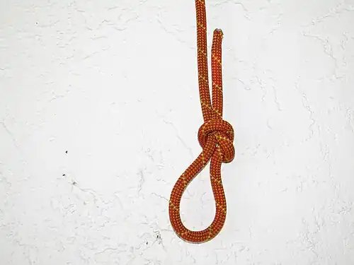
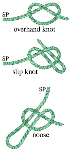
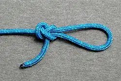
A noose is a loop at the end of a rope in which the knot tightens under load and can be loosened without untying the knot. The knot can be used to secure a rope to a post, pole, or animal but only where the end is in a position that the loop can be passed over.
Tying
The noose knot is a slipped version of the overhand knot
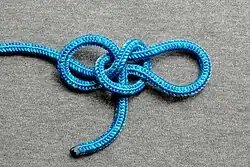
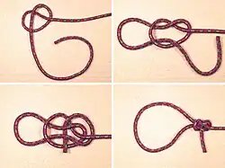
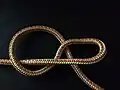
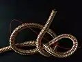
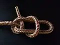
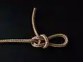
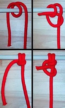
The knot is tied by forming a turn in the end of a rope, and then passing a bight in the standing part through. The noose knot is a slipped version of the overhand knot.
Use in hanging
The knot most closely associated with execution is the hangman’s knot, which is also known as the “hangman’s noose”. Tying is similar to the original noose, but many turns are wrapped around the loop. The reason for this was to make the hanging more humane, as it would break the person’s neck, killing the person instantly, rather than strangling them to death. A similar method is also commonly used for suicide.
Use in intimidation and hate-based racial politics
In the United States, a noose is sometimes left as a message in order to intimidate people, as it was the main object used in segregation era lynchings.[2][3] In 2022, a bill to make lynching a federal hate crime was passed.[4] It is illegal to display a noose in a threatening manner in Virginia,[5] New York and Connecticut.[6]
Austin Reed Edenfield, a former student of the University of Mississippi, pled guilty in 2016 to a federal civil-rights crime, acknowledging that he and Graeme Phillip Harris had tied a noose and a flag of Georgia around the neck of a statue honoring James Meredith, the university’s first African-American student.[7] Harris was sentenced to prison and Edenfield to probation and community service.[8]
In September 2019, Andrew M. Smith, a University of Illinois student, was arrested for placing a noose in a campus elevator. “The incident [came] just months after black employees filed a class-action lawsuit against the campus, alleging they faced racial harassment and were exposed to threats of racial violence, such as nooses, swastikas, KKK garb, racist graffiti, and confederate flags.”[9] He was sentenced to supervision, public service, and a $75 fine.[10]
In November 2022, a noose was found on an Obama Presidential Center construction site.[11]
In July 2025, a noose was found during construction at the New Nissan Stadium.[12]
Bubba Wallace incident
In July 2020 a garage assigned to African-American NASCAR driver Bubba Wallace had been found to contain a “garage door pull rope fashioned like a noose”. After the discovery, which was made by a crew member for Richard Petty Motorsports at the Alabama racetrack, NASCAR was alerted and contacted the FBI, which sent 15 agents to the track to investigate. After the FBI investigation the authorities said the rope had been hanging there since last fall and thus was not a hate crime targeting Wallace. The agencies said no crime was committed and the evidence did not support federal charges.[13][14] The actions of NASCAR, especially NASCAR president Steve Phelps’s claim of it being a hate crime without investigation have been criticized.[15] Holman W. Jenkins Jr. on The Wall Street Journal claimed the controversy and media furor concerning the incident could have been prevented by not contacting the FBI and NASCAR authorities quickly checking the video surveillance by themselves, since NASCAR already tightly controls and surveils access to its garages.[16]
↑Melendez, Pilar (September 3, 2019). “University of Illinois Student Charged With Hate Crime After Noose Found Hanging in Dorm Elevator: Officials”. Daily Beast.
This article is adapted from “Noose” on Wikipedia, written by its contributors, and used under CC BY-SA 4.0. Text on this page is available under the same licence. Source snapshot: Wikipedia via Kiwix, 2026-07-20.
In the mathematical field of knot theory, the Arf invariant of a knot, named after Cahit Arf, is a knot invariant obtained from a quadratic form associated to a Seifert surface. If F is a Seifert surface of a knot, then the homology group H1(F, Z/2Z) has a quadratic form whose value is the number of full twists mod 2 in a neighborhood of an embedded circle representing an element of the homology group. The Arf invariant of this quadratic form is the Arf invariant of the knot.
Definition by Seifert matrix
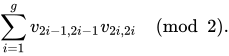
Let be a Seifert matrix of the knot, constructed from a set of curves on a Seifert surface of genus g which represent a basis for the first homology of the surface. This means that V is a 2g × 2g matrix with the property that V − VT is a symplectic matrix. The Arf invariant of the knot is the residue of
Specifically, if , is a symplectic basis for the intersection form on the Seifert surface, then
where lk is the link number and denotes the positive pushoff of a.
Definition by pass equivalence
This approach to the Arf invariant is due to Louis Kauffman.
We define two knots to be pass equivalent if they are related by a finite sequence of pass-moves.[1]
Every knot is pass-equivalent to either the unknot or the trefoil; these two knots are not pass-equivalent and additionally, the right- and left-handed trefoils are pass-equivalent.[2]
Now we can define the Arf invariant of a knot to be 0 if it is pass-equivalent to the unknot, or 1 if it is pass-equivalent to the trefoil. This definition is equivalent to the one above.
Definition by partition function
Vaughan Jones showed that the Arf invariant can be obtained by taking the partition function of an Ising model on a knot diagram.[3]
Definition by Alexander polynomial
This approach to the Arf invariant is by Raymond Robertello.[4] Let
be the Alexander polynomial of the knot. Then the Arf invariant is the residue of
modulo 2, where r = 0 for n odd, and r = 1 for n even.
Kunio Murasugi[5] proved that the Arf invariant is zero if and only if Δ(−1) ≡ ±1 modulo 8.
Arf as knot concordance invariant
From the Fox-Milnor criterion, which tells us that the Alexander polynomial of a slice knot factors as for some polynomial with integer coefficients, we know that the determinant of a slice knot is a square integer. As is an odd integer, it has to be congruent to 1 modulo 8. Combined with Murasugi’s result, this shows that the Arf invariant of a slice knot vanishes.
↑Robertello, Raymond, An Invariant of Knot Corbordism, Communications on Pure and Applied Mathematics, Volume 18, pp. 543–555, 1965
↑Murasugi, Kunio, The Arf Invariant for Knot Types, Proceedings of the American Mathematical Society, Vol. 21, No. 1. (Apr., 1969), pp. 69–72
References
Kauffman, Louis H. (1983). Formal knot theory. Mathematical notes. Vol.30. Princeton University Press. ISBN0-691-08336-3.
Kauffman, Louis H. (1987). On knots. Annals of Mathematics Studies. Vol.115. Princeton University Press. ISBN0-691-08435-1.
Kirby, Robion (1989). The topology of 4-manifolds. Lecture Notes in Mathematics. Vol.1374. Springer-Verlag. ISBN0-387-51148-2.
This article is adapted from “Arf invariant of a knot” on Wikipedia, written by its contributors, and used under CC BY-SA 4.0. Text on this page is available under the same licence. Source snapshot: Wikipedia via Kiwix, 2026-07-20.
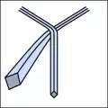
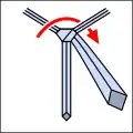
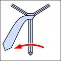
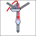
The Nicky knot is a way of tying a necktie. It is a self-releasing version of the Pratt knot.[1] Like the Pratt knot, it is tied inside-out. It originated in Milan, Italy, and may have been named after Nikita Khrushchev after he visited the city. The knot is larger than the Four-in-hand knot and smaller than the Half-Windsor knot.[2]
This article is adapted from “Nicky knot” on Wikipedia, written by its contributors, and used under CC BY-SA 4.0. Text on this page is available under the same licence. Source snapshot: Wikipedia via Kiwix, 2026-07-20.
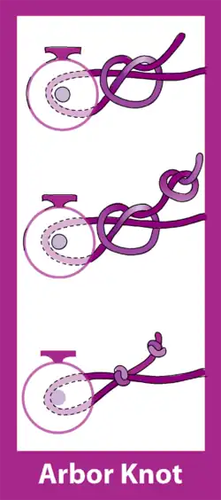
The Arbor knot is a typical fishers’ knot. Its primary use is to attach fishing line to the arbor of a fishing reel.
It has also gained popularity (often under the name “Canadian Jam Knot” or nicknamed “bushcraft zip tie”) as a general binding knot to tie down a roll of e.g. a sleeping bag, or to begin a lashing.[1]
Tying
An arbor knot is tied by first passing the line around the reel arbor. The tag end is then tied in an overhand knot around the running line. Finally, an overhand knot is tied in the tag end. When tightened, the overhand knot in the tag end jams against the overhand knot tied around the running line.[2]
This article is adapted from “Arbor knot” on Wikipedia, written by its contributors, and used under CC BY-SA 4.0. Text on this page is available under the same licence. Source snapshot: Wikipedia via Kiwix, 2026-07-20.
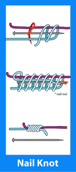
The nail knot, also known as the tube knot or gryp knot, is used in fly fishing to attach the leader to the main fishing line. The knot has been described as “The best known knot for tying a
permanent leader butt of monofilament to a fly line”[1] and “the most satisfactory means of attaching a leader butt to a fly line.” [2] Fly fishing author Sheridan Anderson recommended coating the nail knot with rubberized glue to prevent the knot from hanging up on the guides of the fishing pole.[3]
The nail knot got its name because a nail or similar object such as a narrow straw is inserted as a guide when tying the knot. To tie the nail knot by hand is widely described as very difficult; therefore some anglers use a nail knot-tying tool. Such a tool can be fashioned from a partially straightened paper clip.[1] Commercial versions of nail knot tools are also available. One example is made by Tie-Fast.[4]
This article is adapted from “Nail knot” on Wikipedia, written by its contributors, and used under CC BY-SA 4.0. Text on this page is available under the same licence. Source snapshot: Wikipedia via Kiwix, 2026-07-20.
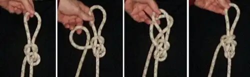
An angler’s loop, otherwise known as a perfection loop, is a type of knot which forms a fixed loop. Useful for fine or slippery line, it is one of the few loop knots which holds well in bungee cord. It is quite secure, but it jams badly and is not suitable if the knot will need to be untied. [1]
it may be tied through an object (typically a ring).
Untightened angler’s loopMethod of tying the angler’s loop through an object
Start with a loop near the working end
Continue with two loops around standing end
one large and one small in the middle
Pull the large loop over the small (working end) and through the first loop
Tighten pulling in all three directions.
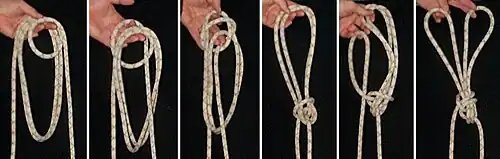
Angler’s loop may be tied around the hand, it may also be tied this way one handed, or with several loops if need be:
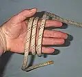
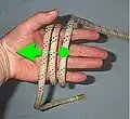
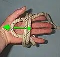
Hold the working end, loop the standing end 3 times around the palm
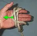
Pull the outmost loop inwards under the first two
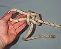
Pull the next outmost over the one(s) in the middle and under the now innermost loop
Pull the now innermost loop(s) and the standing end to tighten.
Done.
Angler’s loop may be locked additionally with half hitches
Locked simple loop A half hitch around the loops root locks it
Angler’s loop may be fashioned with several loops (then locking may be necessary)
with several loops and locked first the loops in desired size, last loop is for the knot and may be smaller. half hitches around the loops roots locks them.
A version with an additional locking turn of the tail called Double Dragon is shown in this video:
This article is adapted from “Angler's loop” on Wikipedia, written by its contributors, and used under CC BY-SA 4.0. Text on this page is available under the same licence. Source snapshot: Wikipedia via Kiwix, 2026-07-20.
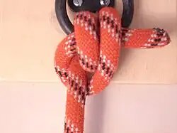
The anchor bend is a knot used for attaching a rope to a ring or similar termination. The name is a misnomer, as it is technically not a bend, but a hitch.
Origins
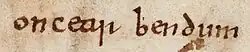
“oncear bendum,” an early evidence of use of anchor bends by Anglo-Saxons from Beowulf
Its name originates from the time when “bend” was understood to simply mean “tie to”; today, a bend strictly refers to a knot that joins two lines.
Techniques
While the knot can become jammed in some modern materials, it is usually easily untied after moderate loads; it can be made more resistant to jamming by taking an extra turn around the object—this will make for a one-diameter longer span of the end to reach around the standing part to be tucked (although in a case of tying to a small shackle or link of a chain, this might not be possible). It is the accepted knot for attaching anchors (or more usually anchor chains) to warps. The knot is very similar to a round turn and two half hitches except that the first half hitch is passed under the turn. In many everyday uses, the finishing half-hitch need not be made; alternatively, one might seek surer security by tying off the end with a strangle knot to the standing part.
Anchor bend step by step, with a finishing half hitch.
Grog. “Anchor Bend”. Animated Knots. Retrieved May 5, 2013.
This article is adapted from “Anchor bend” on Wikipedia, written by its contributors, and used under CC BY-SA 4.0. Text on this page is available under the same licence. Source snapshot: Wikipedia via Kiwix, 2026-07-20.
In mathematics, the Möbius energy of a knot is a particular knot energy, i.e., a functional on the space of knots. It was discovered by Jun O’Hara, who demonstrated that the energy blows up as the knot’s strands get close to one another.[1] This is a useful property because it prevents self-intersection and ensures the result under gradient descent is of the same knot type.
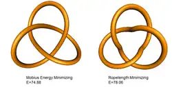
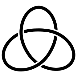
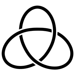
Pictures of two trefoil knots, with different Möbius energies. The knot on the left has a Möbius energy of 74.88, close to the minimum of 74.41 [2]. The knot on the right has close to the minimum ropelength, but a higher Möbius energy of 78.06.
Invariance of Möbius energy under Möbius transformations was demonstrated by Michael Freedman, Zheng-Xu He, and Zhenghan Wang (1994) who used it to show the existence of a energy minimizer in each isotopy class of a prime knot. They also showed the minimum energy of any knot conformation is achieved by a round circle.[3]
Conjecturally, there is no energy minimizer for composite knots. Robert B. Kusner and John M. Sullivan have done computer experiments with a discretized version of the Möbius energy and concluded that there should be no energy minimizer for the knot sum of two trefoils (although this is not a proof).
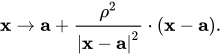
Recall that the Möbius transformations of the 3-sphere are the ten-dimensional group of angle-preserving diffeomorphisms generated by inversion in 2-spheres. For example, the inversion in the sphere is defined by
Consider a rectifiable simple curve in the Euclidean
3-space , where belongs to or . Define its energy by
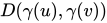
where is the shortest arc
distance between
and on the curve. The second term of the
integrand is called a
regularization. It is easy to see that is
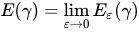
independent of parametrization and is unchanged if is changed by a similarity of . Moreover, the energy of any line is 0, the energy of any circle is . In fact, let us use the arc-length parameterization. Denote by the length of the curve . Then
Let denote a unit circle. We have
and consequently,
since .
Knot invariant
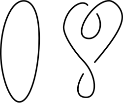
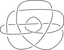
On the left, the unknot, and a knot equivalent to it. It can be more difficult to determine whether complex knots, such as the one on the right, are equivalent to the unknot.
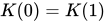
A knot is created by beginning with a one-dimensional line segment, wrapping it around itself arbitrarily, and then fusing its two free ends together to form a closed loop.[4] Mathematically, we can say a knot is an injective and continuous function with . Topologists consider knots and other entanglements such as links and braids to be equivalent if the knot can be pushed about smoothly, without intersecting itself, to coincide with another knot. The idea of knot equivalence is to give a precise definition of when two knots should be considered the same even when positioned quite differently in space. A mathematical definition is that two knots are equivalent if there is an orientation-preserving homeomorphism with , and this is known to be equivalent to existence of ambient isotopy.
The basic problem of knot theory, the recognition problem, is determining the equivalence of two knots. Algorithms exist to solve this problem, with the first given by Wolfgang Haken in the late 1960s.[5] Nonetheless, these algorithms can be extremely time-consuming, and a major issue in the theory is to understand how hard this problem really is.[5] The special case of recognizing the unknot, called the unknotting problem, is of particular interest.[6]
We shall picture a knot by a smooth curve rather than by a polygon. A knot will be represented by a planar diagram. The singularities of the planar diagram will be called crossing points and the regions into which it subdivides the plane regions of the diagram. At each crossing point, two of the four corners will be dotted to indicate which branch through the crossing point is to be thought of as one passing under the other. We number any one region at random, but shall fix the numbers of all remaining regions such that whenever we cross the curve from right to left we must pass from region number to the region number . Clearly, at any crossing point , there are two opposite corners of the same number and two opposite corners of the numbers and , respectively. The number is referred as the index of . The crossing points are distinguished by two types: the right handed and the left handed, according to which branch through the point passes under or behind the other. At any crossing point of index two dotted corners are of numbers and , respectively, two undotted ones of numbers and . The index of any corner of any region of index is one element of . We wish to distinguish one type of knot from another by knot invariants. There is one invariant which is quite simple. It is Alexander polynomial with integer coefficient. The Alexander polynomial is symmetric with degree : for all knots of crossing points. For example, the invariant of an unknotted curve is 1, of an trefoil knot is .
The left handed trefoil knot.
The right handed trefoil knot.
Let
denote the standard surface element of .
We have
For the knot :[0,1]\rightarrow \mathbb {R} ^{3}}
, ,
does not change, if we change the knot in its equivalence class.
Möbius Invariance Property
Let be a closed curve in and a Möbius transformation of . If is contained in then . If passes through then .
Theorem A. Among all rectifiable loops , round circles have the least energy and any of least energy parameterizes a round circle.
Proof of Theorem A. Let be a Möbius transformation sending a point of to infinity. The energy with equality holding if and only if is a straight line. Apply the Möbius invariance property we complete the proof.
Proof of Möbius Invariance Property. It is sufficient to consider how , an inversion in a sphere, transforms energy. Let be the arc length parameter of a rectifiable closed curve , . Let
1
and
2
Clearly, and . It is a short calculation (using the law of cosines) that the first terms transform correctly, i.e.,
Since is arclength for , the regularization term of (1) is the elementary integral
3
Let be an arclength parameter for .
Then where denotes the linear expansion factor of . Since is a Lipschitz function and is smooth, is Lipschitz, hence, it has weak derivative .
For the second assertion, let send a point of to infinity. In this case and, thus, the constant term 4 in (5) disappears.
Freedman–He–Wang conjecture
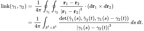
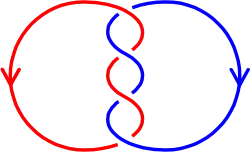
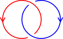
The Freedman–He–Wang conjecture (1994) stated that the Möbius energy of nontrivial links in is minimized by the stereographic projection of the standard Hopf link. This was proved in 2012 by Ian Agol, Fernando C. Marques and André Neves, by using Almgren–Pitts min-max theory.[7] Let , be a link of 2 components, i.e., a pair of rectifiable closed curves in Euclidean three-space with . The Möbius cross energy of the link is defined to be
The numerator of the linking integrand contains a factor of the displacement between two line elements that reduces the cubic distance dependence to a square, similar to the Möbius energy integrand. The linking integrand will be reduced by the dot product of the displacement vector with the cross product of the two tangent vectors of those line elements, which may be unitary at a few locations but is typically less than one. For that reason, . If two circles are unlinked and very far from each other, the cross energy can be made arbitrarily small but nonzero. If the linking number is non-zero, the link is called non-split and for the non-split link, . So we are interested in the minimal energy of non-split links.
Note that the definition of the energy extends
to any 2-component link in . The Möbius energy has the remarkable property of being invariant under conformal transformations of . This property is explained as follows. Let denote a conformal map. Then This condition is called the conformal invariance property of the Möbius cross energy.
Main Theorem. Let , be a non-split link of 2 components link. Then .
Moreover, if then there exists a conformal map such that and (the standard Hopf link up to orientation and reparameterization).
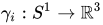
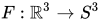
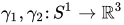
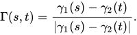
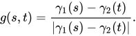
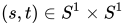
Given two non-intersecting differentiable curves , define the Gauss map from the torus to the sphere by
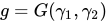
The Gauss map of a link in , denoted by , is the Lipschitz map defined by
We denote an open ball in , centered at with radius , by . The boundary of this ball is denoted by . An intrinsic open ball of , centered at with radius , is denoted by .
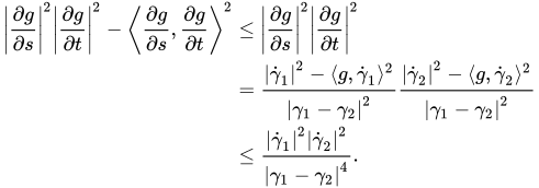
We have
Thus,
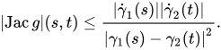
It follows that for almost every ,
If equality holds at , then
If the link is contained in an oriented affine hyperplane with unit normal vector compatible with the orientation, then
References
Adams, Colin (2004). The Knot Book: An Elementary Introduction to the Mathematical Theory of Knots. American Mathematical Society. ISBN9780821836781.
↑Freedman, Michael H.; He, Zheng-Xu; Wang, Zhenghan (January 1994). “Möbius energy of knots and unknots”. Annals of Mathematics. Second Series. 139 (1): 1–50. doi:10.2307/2946626. JSTOR2946626. MR1259363.
↑Hoste, Jim (December 2005). “The enumeration and classification of knots and links”. In William W. Menasco; Morwen B. Thistlethwaite (eds.). Handbook of Knot Theory(PDF). Amsterdam: Elsevier. pp.209–232. doi:10.1016/B978-044451452-3/50006-X. ISBN9780444514523.
↑Agol, Ian; Marques, Fernando C.; Neves, André (2012). “Min-max theory and the energy of links”. arXiv:1205.0825 [math.GT].
This article is adapted from “Möbius energy” on Wikipedia, written by its contributors, and used under CC BY-SA 4.0. Text on this page is available under the same licence. Source snapshot: Wikipedia via Kiwix, 2026-07-20.
The concept of alternating planar algebras first appeared in the work of Hernando Burgos-Soto[1] on the Jones polynomial of alternating tangles. Alternating planar algebras provide an appropriate algebraic framework for other knot invariants in cases the elements involved in the computation are alternating. The concept has been used in extending to tangles some properties of Jones polynomial and Khovanov homology of alternating links.
Definition
An alternating planar algebra is an oriented planar algebra, where the -input planar arc diagrams satisfy the following conditions:
The number of strings ending on the external boundary of is greater than 0.
There is complete connection among input discs of the diagram and its arcs, namely, the union of the diagram arcs and the boundary of the internal holes is a connected set.
The in- and out-strings alternate in every boundary component of the diagram.
A planar arc diagram like this has been denominated type- planar diagram.
Applications
There are two known applications of the concept of alternating planar algebra.
It was used for extend to tangles the property that states that the Jones Polynomial of an alternating link is an alternating polynomial.
It was used for extend to tangles a result about the Khovanov homology that states that The Khovanov homology of an alternating link is supported in two lines.[2]
Notes
↑Burgos-Soto, Hernando (2010). “The Jones Polynomial of Alternating Tangles”. Journal of Knot Theory and Its Ramifications. 19 (11): 1487–1505. arXiv:0807.2600. doi:10.1142/s0218216510008510. S2CID13993750.
↑Bar-Natan, Dror; Burgos-Soto, Hernando (2014). “Khovanov homology for alternating tangles”. Journal of Knot Theory and Its Ramifications. 23 (2): 1450013. arXiv:1305.1695. doi:10.1142/s0218216514500138. S2CID119237571.
This article is adapted from “Alternating planar algebra” on Wikipedia, written by its contributors, and used under CC BY-SA 4.0. Text on this page is available under the same licence. Source snapshot: Wikipedia via Kiwix, 2026-07-20.
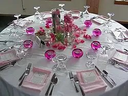
A table with ten place settings. There are 3120 different ways in which five male-female couples can sit at this table such that men and women alternate and nobody sits next to their partner.
In combinatorial mathematics, the ménage problem or problème des ménages asks for the number of different ways in which it is possible to seat a set of male-female couples at a round dining table so that men and women alternate and nobody sits next to his or her partner. (Ménage is the French word for “household”, referring here to a male-female couple.) This problem was formulated in 1891 by Édouard Lucas and independently, a few years earlier, by Peter Guthrie Tait in connection with knot theory.[1] For a number of couples equal to 3, 4, 5, … the number of seating arrangements is
12, 96, 3120, 115200, 5836320, 382072320, 31488549120, … (sequence A059375 in the OEIS).
Mathematicians have developed formulas and recurrence equations for computing these numbers and related sequences of numbers. Along with their applications to etiquette and knot theory, these numbers also have a graph theoretic interpretation: they count the numbers of matchings and Hamiltonian cycles in certain families of graphs.
Touchard’s formula
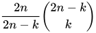
Let Mn denote the number of seating arrangements for n couples. Touchard (1934) derived the formula
Much subsequent work has gone into alternative proofs for this formula and into various generalized versions of the problem.
A different umbral formula for Mn involving Chebyshev polynomials of first kind was given by Wyman & Moser (1958).
Ménage numbers and ladies-first solutions
There are 2×n! ways of seating the women: there are two sets of seats that can be arranged for the women, and there are n! ways of seating them at a particular set of seats. For each seating arrangement for the women, there are
ways of seating the men; this formula simply omits the 2×n! factor from Touchard’s formula. The resulting smaller numbers (again, starting from n=3),
1, 2, 13, 80, 579, 4738, 43387, 439792, … (sequence A000179 in the OEIS)
are called the ménage numbers. The factor is the number of ways of forming k non-overlapping pairs of adjacent seats or, equivalently, the number of matchings of k edges in a cycle graph of 2n vertices. The expression for An is the immediate result of applying the principle of inclusion–exclusion to arrangements in which the people seated at the endpoints of each edge of a matching are required to be a couple.
Until the work of Bogart & Doyle (1986), solutions to the ménage problem took the form of first finding all seating arrangements for the women and then counting, for each of these partial seating arrangements, the number of ways of completing it by seating the men away from their partners. Bogart and Doyle argued that Touchard’s formula may be derived directly by considering all seating arrangements at once rather than by factoring out the participation of the women.[2] However, Kirousis & Kontogeorgiou (2018) found the even more straightforward ladies-first solution described above by making use of a few of Bogart and Doyle’s ideas (although they took care to recast the argument in non-gendered language).
The ménage numbers satisfy the recurrence relation[3]
from which the ménage numbers themselves can easily be calculated.
Graph-theoretical interpretations
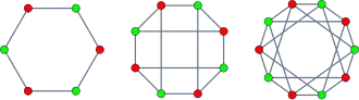
Crown graphs with six, eight, and ten vertices. The outer cycle of each graph forms a Hamiltonian cycle; the eight and ten vertex graphs also have other Hamiltonian cycles.
Solutions to the ménage problem may be interpreted in graph-theoretic terms, as directed Hamiltonian cycles in crown graphs. A crown graph is formed by removing a perfect matching from a complete bipartite graph Kn,n; it has 2n vertices of two colors, and each vertex of one color is connected to all but one of the vertices of the other color. In the case of the ménage problem, the vertices of the graph represent men and women, and the edges represent pairs of men and women who are allowed to sit next to each other. This graph is formed by removing the perfect matching formed by the male-female couples from a complete bipartite graph that connects every man to every woman. Any valid seating arrangement can be described by the sequence of people in order around the table, which forms a Hamiltonian cycle in the graph. However, two Hamiltonian cycles are considered to be equivalent if they connect the same vertices in the same cyclic order regardless of the starting vertex, while in the ménage problem the starting position is considered significant: if, as in Alice’s tea party, all the guests shift their positions by one seat, it is considered a different seating arrangement even though it is described by the same cycle. Therefore, the number of oriented Hamiltonian cycles in a crown graph is smaller by a factor of 2n than the number of seating arrangements,[5] but larger by a factor of (n−1)! than the ménage numbers. The sequence of numbers of cycles in these graphs (as before, starting at n=3) is
2, 12, 312, 9600, 416880, 23879520, 1749363840, … (sequence A094047 in the OEIS).
A second graph-theoretic description of the problem is also possible. Once the women have been seated, the possible seating arrangements for the remaining men can be described as perfect matchings in a graph formed by removing a single Hamiltonian cycle from a complete bipartite graph; the graph has edges connecting open seats to men, and the removal of the cycle corresponds to forbidding the men to sit in either of the open seats adjacent to their wives. The problem of counting matchings in a bipartite graph, and therefore a fortiori the problem of computing ménage numbers, can be solved using the permanents of certain 0-1 matrices. In the case of the ménage problem, the matrix arising from this view of the problem is the circulant matrix in which all but two adjacent elements of the generating row equal 1.[6]
Knot theory
Tait’s motivation for studying the ménage problem came from trying to find a complete listing of mathematical knots with a given number of crossings, say n. In Dowker notation for knot diagrams, an early form of which was used by Tait, the 2n points where a knot crosses itself, in consecutive order along the knot, are labeled with the 2n numbers from 1 to 2n. In a reduced diagram, the two labels at a crossing cannot be consecutive, so the set of pairs of labels at each crossing, used in Dowker notation to represent the knot, can be interpreted as a perfect matching in a graph that has a vertex for every number in the range from 1 to 2n and an edge between every pair of numbers that has different parity and are non-consecutive modulo 2n. This graph is formed by removing a Hamiltonian cycle (connecting consecutive numbers) from a complete bipartite graph (connecting all pairs of numbers with different parity), and so it has a number of matchings equal to a ménage number. For alternating knots, this matching is enough to describe the knot diagram itself; for other knots, an additional positive or negative sign needs to be specified for each crossing pair to determine which of the two strands of the crossing lies above the other strand.
However, the knot listing problem has some additional symmetries not present in the ménage problem: one obtains different Dowker notations for the same knot diagram if one begins the labeling at a different crossing point, and these different notations should all be counted as representing the same diagram. For this reason, two matchings that differ from each other by a cyclic permutation should be treated as equivalent and counted only once. Gilbert (1956) solved this modified enumeration problem, showing that the number of different matchings is
1, 2, 5, 20, 87, 616, 4843, 44128, 444621, … (sequence A002484 in the OEIS).
See also
Oberwolfach problem, a different mathematical problem involving the arrangement of diners at tables
Problème des rencontres, a similar problem involving partial derangements
Bong, Nguyen-Huu (1998), “Lucas numbers and the menage problem”, International Journal of Mathematical Education in Science and Technology, 29 (5): 647–661, Bibcode:1998IJMES..29..647B, doi:10.1080/0020739980290502, MR1649926.
Canfield, E. Rodney; Wormald, Nicholas C. (1987), “Ménage numbers, bijections and P-recursiveness”, Discrete Mathematics, 63 (2–3): 117–129, doi:10.1016/0012-365X(87)90002-1, MR0885491.
Dörrie, Heinrich (1965), “Lucas’ Problem of the Married Couples”, 100 Great Problems of Elementary Mathematics, translated by Antin, David, Dover, pp.27–33, ISBN978-0-486-61348-2.
Dutka, Jacques (1986), “On the problème des ménages”, The Mathematical Intelligencer, 8 (3): 18–33, doi:10.1007/BF03025785, MR0846991, S2CID116433056.
Eades, Peter; Praeger, Cheryl E.; Seberry, Jennifer R. (1983), “Some remarks on the permanents of circulant (0,1) matrices”, Utilitas Mathematica, 23: 145–159, MR0703136.
Gilbert, E. N. (1956), “Knots and classes of ménage permutations”, Scripta Mathematica, 22: 228–233, MR0090568.
Henderson, J. R. (1975), “Permanents of (0,1)-matrices having at most two zeros per line”, Canadian Mathematical Bulletin, 18 (3): 353–358, doi:10.4153/CMB-1975-064-6, MR0399127.
Holst, Lars (1991), “On the ‘problème des ménages’ from a probabilistic viewpoint”, Statistics and Probability Letters, 11 (3): 225–231, doi:10.1016/0167-7152(91)90147-J, MR1097978.
Kaplansky, Irving (1943), “Solution of the problème des ménages”, Bulletin of the American Mathematical Society, 49 (10): 784–785, doi:10.1090/S0002-9904-1943-08035-4, MR0009006.
Kaplansky, Irving; Riordan, J. (1946), “The problème des ménages”, Scripta Mathematica, 12: 113–124, MR0019074.
Kirousis, L.; Kontogeorgiou, G. (2018), “102.18 The problème des ménages revisited”, The Mathematical Gazette, 102 (553): 147–149, arXiv:1607.04115, doi:10.1017/mag.2018.27, S2CID126036427.
Laisant, Charles-Ange (1891), “Sur deux problèmes de permutations”, Vie de la société, Bulletin de la Société Mathématique de France (in French), 19: 105–108.
Lucas, Édouard (1891), Théorie des Nombres, Paris: Gauthier-Villars, pp.491–495.
This article is adapted from “Ménage problem” on Wikipedia, written by its contributors, and used under CC BY-SA 4.0. Text on this page is available under the same licence. Source snapshot: Wikipedia via Kiwix, 2026-07-20.



















![{\displaystyle E(\gamma )=\int _{-\ell /2}^{\ell /2}{}dx\int _{x-\ell /2}^{x+\ell /2}\left[{1 \over |\gamma (x)-\gamma (y)|^{2}}-{1 \over |x-y|^{2}}\right]dy.}](/wp-content/uploads/wiki-images/5e43d9199c18fbaa3d6a68120731f9ea2827e48c-376e7d8d.svg)


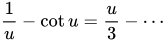
![{\displaystyle {\begin{aligned}E(\gamma _{0})&=\int _{-\pi }^{\pi }{}dx\int _{x-\pi }^{x+\pi }\left[{1 \over \left(2\sin {\tfrac {1}{2}}(x-y)\right)^{2}}-{1 \over |x-y|^{2}}\right]dy\\&=4\pi \int _{0}^{\pi }\left[{1 \over \left(2\sin(y/2)\right)^{2}}-{1 \over |y|^{2}}\right]dy\\&=2\pi \int _{0}^{\pi /2}\left[{1 \over \sin ^{2}y}-{1 \over |y|^{2}}\right]dy\\&=2\pi \left[{1 \over u}-\cot u\right]_{u=0}^{\pi /2}=4\end{aligned}}}](/wp-content/uploads/wiki-images/a6f5bb41c38af406eadd5473e037bb9b040c7c42-8e650a39.svg)

![{\displaystyle K\colon [0,1]\to \mathbb {R} ^{3}}](/wp-content/uploads/wiki-images/3527c328346ff511b17bd2fe2ae5f3504df3d2e9-11b6d444.svg)








![{\displaystyle \gamma :[0,1]\rightarrow \mathbb {R} ^{3}}](/wp-content/uploads/wiki-images/f571fb855af7f0a45d001b9e9f758d85fe339573-e8c55395.svg) ,
, 

![{\displaystyle +\int _{t_{1}<t_{2}<t_{3},{\boldsymbol {x}}\in \mathbb {R} ^{3}\setminus \gamma ([0,1])}\omega (\gamma (t_{1})-{\boldsymbol {x}})\wedge \omega (\gamma (t_{2})-{\boldsymbol {x}})\wedge \omega (\gamma (t_{3})-{\boldsymbol {x}})}](/wp-content/uploads/wiki-images/6c559a97bed84443bf754509af5182cb9d6b807f-bd8a7298.svg)















![{\displaystyle \int _{u=0}^{\ell }\left[2\int _{v=\varepsilon }^{\ell /2}{\frac {1}{v^{2}}}\,dv\right]\,du=4-{\frac {2\ell }{\varepsilon }}.}](/wp-content/uploads/wiki-images/42db793581695c97a4d59ddb7b30bb809b550904-e95ad8c9.svg)






![{\displaystyle {\begin{aligned}{\rm {{regularization}(2)=}}&\int _{u\in \mathbf {R} /\ell \mathbf {Z} }\left[\int _{|v-u|\geq \varepsilon }{\frac {|(I\circ \gamma )'(v)|\,dv}{D(I\circ \gamma (u),I\circ \gamma (v))^{2}}}\right]|(I\circ \gamma )'(u)|\,du\\=&\int _{\mathbf {R} /\ell \mathbf {Z} }\left[{\frac {4}{L}}-{\frac {1}{\varepsilon _{+}}}-{\frac {1}{\varepsilon _{-}}}\right]\,ds,\end{aligned}}}](/wp-content/uploads/wiki-images/6d4250b6416df50fc0c0f611e4713d333ce44218-13dca44f.svg)




![{\displaystyle {\begin{aligned}{\frac {1}{\varepsilon _{+}}}=&{\frac {1}{f(u)\varepsilon }}\left[{1+{\varepsilon \over f(u)}\int _{0}^{1}(1-t)f'(u+\varepsilon t)\,dt}\right]^{-1}\\=&{\frac {1}{f(u)\varepsilon }}\left[1-{\frac {\varepsilon }{f(u)}}\int _{0}^{1}(1-t)f'(u+\varepsilon t)\,dt+O(\varepsilon ^{2})\right]\\=&{\frac {1}{f(u)\varepsilon }}-{\frac {1}{f(u)^{2}}}\int _{0}^{1}(1-t)f'(u+\varepsilon t)\,dt+O(\varepsilon ).\end{aligned}}}](/wp-content/uploads/wiki-images/0fab1a5cd3107d92025983129dddcf59ea4bdba2-114145ae.svg)

![{\displaystyle {\begin{aligned}{\rm {{regularization}\ (2)=}}&4-\int _{0}^{\ell }{\frac {2}{\varepsilon }}\,du+O(\varepsilon )\\&+\int _{u=0}^{\ell }\int _{t=0}^{1}{\frac {(1-t)}{f(u)}}[f'(u+\varepsilon t)-f'(u-\varepsilon t)]\,du\,dt\\=&4-{\frac {2\ell }{\varepsilon }}+O(\varepsilon ).\end{aligned}}}](/wp-content/uploads/wiki-images/15f10d9d42ce306698c5c49adc4c5760ae3c6c97-deb30794.svg)