Category: Knots

  • Dropper loop

    Dropper loop knot
    Dropper loop
    Names Dropper loop knot, blood dropper loop [1] blood loop dropper knot [2]
    Category Loop
    Typical use Fishing
    ABoK
    Instructions

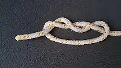
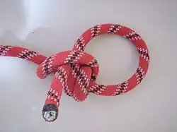
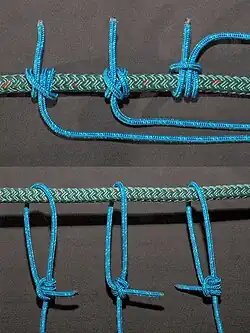
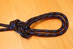
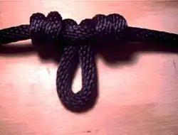
    The dropper loop is a type of loop knot often used on multi-hook fishing lines. It can be created in the middle of a long line and forms a loop which is off to the side of the line.

    Techniques

    There are two main methods of tying the dropper loop.

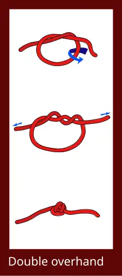
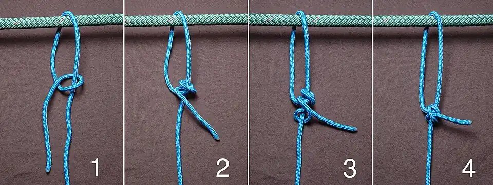
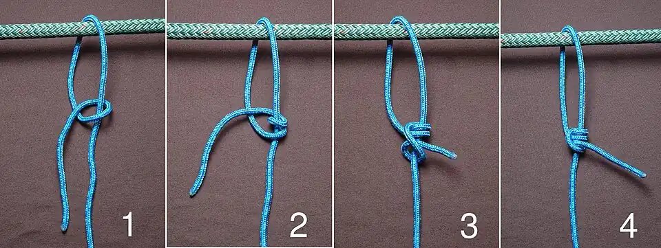
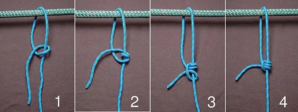
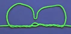
    1. Gather a loop and then twist it around the overlap a few times
    2. Form the loop and then use a matchstick to twist up the overlap.

    Finally drop the loop through the central twist.

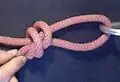
    Dropper loop
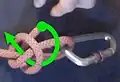
    Dropper Loop being formed

    See also

    References

    1. Handbook of Knots — Des Pawson — p125 — ISBN 1-4053-0467-7
    2. The complete guide to knots and knot tying — Geoffrey Budworth — p.182 — ISBN 0-7548-0422-4

    This article is adapted from “Dropper loop” on Wikipedia, written by its contributors, and used under CC BY-SA 4.0. Text on this page is available under the same licence. Source snapshot: Wikipedia via Kiwix, 2026-07-20.

  • The 85 Ways to Tie a Tie

    The 85 Ways to Tie a Tie
    The 85 Ways to Tie a Tie
    Author Thomas Fink and Yong Mao
    Publisher Fourth Estate
    Publication date November 4, 1999
    ISBN 1-84115-249-8
    OCLC 59397523

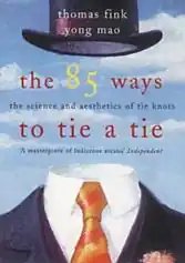
    The 85 Ways to Tie a Tie is a book by Thomas Fink and Yong Mao about the history of the knotted neckcloth, the modern necktie, and how to tie each. It is based on two mathematics papers published by the authors in Nature[1] and Physica A while they were research fellows at Cambridge University’s Cavendish Laboratory.[2] The authors prove that, assuming both the tie and the wearer to be of typical size, there are exactly 85 ways of tying a necktie using the conventional method of wrapping the wide end of the tie around the narrow end. They describe each and highlight those that they determine to be historically notable or aesthetically pleasing.

    It was published by Fourth Estate on November 4, 1999, and subsequently published in nine other languages.

    The mathematics

    The discovery of all possible ways to tie a tie depends on a mathematical formulation of the act of tying a tie. In their papers (which are technical) and book (which is for a lay audience, apart from an appendix), the authors show that necktie knots are equivalent to persistent random walks on a triangular lattice, with some constraints on how the walks begin and end. Thus enumerating tie knots of n moves is equivalent to enumerating walks of n steps. Imposing the conditions of symmetry and balance reduces the 85 knots to 13 aesthetic ones.

    Knot representation

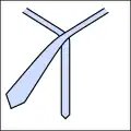
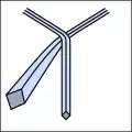
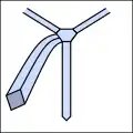
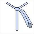
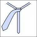
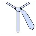
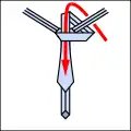
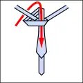
    The basic idea is that tie knots can be described as a sequence of five
    different possible moves, although not all moves can follow each other. These are summarized as follows. All diagrams are as the tie would appear were you wearing it and looking in a mirror.

    • L: left; C: centre; R: right; these must change every move.
    • i: into the diagram; o: out of the diagram; these must alternate.
    • T: through the loop just made.

    With this shorthand, traditional and new knots can be compactly expressed, as below. Note that any knot that begins with an o move must start with the tie turned inside out around the neck.[3]

    • Tie knotting examples.
    • Li beginning.
      Li beginning.
    • Lo beginning.
      Lo beginning.
    • Lo
      Lo
    • Ro
      Ro
    • Li
      Li
    • Ri
      Ri
    • Lo Ri Co T end.
      Lo Ri Co T end.
    • Ro Li Co T end.
      Ro Li Co T end.

    Knots

    Selection criteria

    Of the 85 knots possible with a typical necktie, Fink and Mao selected thirteen as “aesthetic knots” suitable for use. They made their selection based on three criteria: shape, symmetry, and balance.

    Shape

    In Fink and Mao’s classification, each of the 85 tie knots belongs to a particular “class”, which is defined by its total number of moves and its number of centering moves. For example, the four-in-hand is a four-move, one-center knot, while the half-Windsor is a six-move, two-center knot. Knots with fewer centering moves, less than one-third of the total, appear narrower and more elongated, while knots with more centering moves appear wider and more squat. Due to the triangular nature of tie knots, the number of centering moves must necessarily be less than half the total number of moves.

    There are a total of 16 classes, ranging from three moves with one center to nine moves with four centers, but only classes in which the ratio of centering moves to total moves is 1:6 or greater contain an aesthetic knot, eliminating three classes (ten knots) for a remaining 13 classes, with 75 knots. (In the Nature paper, the lower bound was placed at a more restrictive 1:4, eliminating the knot classes containing the Kelvin, Victoria, and Grantchester; this was likely revised specifically in order to include the Victoria/Prince Albert, which has fairly extensive historical documentation.) The most representative knot in each remaining class was then selected on the basis of symmetry and balance.

    Symmetry

    Symmetry in the case of tie knots can refer to two possible qualities: visual symmetry (the extent to which the knot appears to be shaped identically on the left and right side), and mathematical symmetry (the number of L and R moves being as close to equal as possible). Fink and Mao refer to the latter, even though some knots that are slightly asymmetrical (such as the Nicky and the Windsor) appear symmetrical to the eye. Only knots with an equal number of total L and R moves can be mathematically symmetrical, while the remainder of the aesthetic knots will necessarily have one greater L or R move.

    Balance

    Fink and Mao describe balance as “the extent to which the moves are well-mixed”, citing a tighter knot that comes loose less easily as its primary virtue. It is calculated by a particular formula, but can be best understood by the layman as the degree to which the L, R, and C moves are evenly distributed throughout the knotting sequence, and the extent to which the L-R or R-L pattern continues uninterrupted after non-terminal centering moves (which requires a change of winding direction from counterclockwise to clockwise, or vice versa). Each of the aesthetic knots displays these qualities.

    A number of knots have virtually identical variants, which differ by the transposition of L and R pairs. For instance, a variant of the Half-Windsor, Li Ro Ci Lo Ri Co T (Knot 7), is the knot Li Ro Ci Ro Li Co T (Knot 8), sometimes called the co-Half-Windsor. References to the Half-Windsor in the literature sometimes refer to one, sometimes to the other. For the purposes of the book, when a knot has at least one variant (i.e., when two or more knots, at the greatest degree of symmetry for their class, share the same basic structure apart from one or more transposed L-R pairs), the most balanced version is given the standard designation, while the others are labeled as variants, irrespective of qualities such as being self-releasing (coming undone when the narrow end is pulled out). Thus, the more balanced of the two “half-Windsor” knots is given a lower numbering and the name “Half-Windsor”, even though the slightly less balanced “co-Half-Windsor” variant is equally known as the “Half-Windsor” in men’s style literature, and has the benefit of being self-releasing, and the most common way of tying the Windsor knot is called “co-Windsor 3” by Fink and Mao. However, this is not intended to mark an aesthetic preference for one variant over the other(s); as the authors note in their journal articles, “We do not attempt to distinguish between these knots and their counterparts; this much we leave to the sartorial discretion of the reader.”

    Three of the aesthetic knots (the St Andrew, Cavendish, and Grantchester) have the same symmetry and balance values as at least one other knot in their class; in this case, they appear to have been selected based on how evenly they distribute the unbalanced portions throughout the knot. This can be readily seen when one views these knots as combinations of two smaller knots, as the balance values of each component add up to the balance value of the final knot. In unbalanced knots where the balance value is odd, it is broken up so that the more unbalanced portion of the two is placed towards the beginning of the knot. This is probably intended to help the outermost portion of the knot keep its shape and remain tight.

    The 13 aesthetic knots

    The thirteen aesthetic knots described in the book, in order of size, are as follows. Terminal sequences (the final three moves that end in the tying of the knot) are in bold. The knots are sometimes designated by their number alone (e.g., FM2 for the four-in-hand, with FM standing for Fink-Mao). A knot is self-releasing if, when the thin end is pulled out through the knot, no knot is left; as all knots start on the left, a knot is self-releasing if the terminal sequence is Ro Li Co; it is not self-releasing if the terminal sequence is Lo Ri Co. Symmetry and self-releasing are in complementary distribution for knots with the greatest degree of balance for their class.

    Number Sequence Name Self-releasing Symmetric[4]
    1. Lo Ri Co T Small knot No Yes
    2. Li Ro Li Co T Four-in-hand Yes No
    3. Lo Ri Lo Ri Co T Kelvin No Yes
    4. Lo Ci Ro Li Co T Nicky Yes No
    6. Li Ro Li Ro Li Co T Victoria Yes No
    7. Li Ro Ci Lo Ri Co T Half-Windsor No Yes
    12. Lo Ri Lo Ci Ro Li Co T St Andrew Yes No
    18. Lo Ci Ro Ci Lo Ri Co T Plattsburgh No Yes
    23. Li Ro Li Co Ri Lo Ri Co T Cavendish No Yes
    31. Li Co Ri Lo Ci Ro Li Co T Windsor Yes No
    44. Lo Ri Lo Ri Co Li Ro Li Co T Grantchester Yes No
    54. Lo Ri Co Li Ro Ci Lo Ri Co T Hanover No Yes
    78. Lo Ci Ro Ci Lo Ci Ro Li Co T Balthus Yes No

    Three common variant knots are as follows. They are included for their commonality (Pratt, Half-Windsor variant), or for being self-releasing when their more “aesthetic” counterparts are not (Half-Windsor variant, Hanover variant). The Half-Windsor and Hanover variants have the advantage of being both symmetrical and self-releasing, but are less balanced than their counterparts above:

    Number Sequence Name Self-releasing Symmetric[4]
    5. Lo Ci Lo Ri Co T Pratt No No
    8. Li Ro Ci Ro Li Co T Half-Windsor variant Yes Yes
    55. Lo Ri Co Ri Lo Ci Ro Li Co T Hanover variant Yes Yes

    Reviews

    The book was reviewed in Nature,[5] The Daily Telegraph, The Guardian, GQ, Physics World, and others.

    References

    1. Fink, Thomas M.; Yong Mao (1999). “Designing tie knots by random walks” (PDF). Nature. 398 (6722): 31–32. doi:10.1038/17938. Archived from the original (PDF) on 2019-02-22. Retrieved 2024-09-09.
    2. Fink, Thomas M.; Yong Mao (2000). “Tie knots, random walks and topology” (PDF). Physica A. 276 (1–2): 109–121. doi:10.1016/S0378-4371(99)00226-5. Archived from the original (PDF) on 2019-07-17. Retrieved 2024-09-09.
    3. “How to tie a tie – Quick and very easy step by step”. www.ezone57.net. 2023-02-15. Retrieved 2024-05-02.
    4. 1 2 “Encyclopedia of Tie Knots at Thomas Fink’s homepage”. Archived from the original on 2019-12-22. Retrieved 2019-12-22.
    5. Buck, Gregory (2000). “Why not knot right?”. Nature. 403 (6768): 362. doi:10.1038/35000270.

    External links


    This article is adapted from “The 85 Ways to Tie a Tie” on Wikipedia, written by its contributors, and used under CC BY-SA 4.0. Text on this page is available under the same licence. Source snapshot: Wikipedia via Kiwix, 2026-07-20.

  • Dowker–Thistlethwaite notation

    Dowker–Thistlethwaite notation
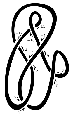
    A knot diagram with crossings labelled for a Dowker sequence

    In the mathematical field of knot theory, the DowkerThistlethwaite (DT) notation or code, for a knot diagram is a sequence of even integers. The notation is named after Clifford Hugh Dowker and Morwen Thistlethwaite, who refined a notation originally due to Peter Guthrie Tait.[1] It is not an invariant of the associated knot.

    Definition

    To generate the Dowker–Thistlethwaite notation, traverse the knot using an arbitrary starting point and direction. Label each of the n crossings with the numbers 1, …, 2n in order of traversal (each crossing is visited and labelled twice), with the following modification: if the label is an even number and the strand followed crosses over at the crossing, then change the sign on the label to be a negative. When finished, each crossing will be labelled a pair of integers, one even and one odd.[2] The Dowker–Thistlethwaite notation is the sequence of even integer labels associated with the labels 1, 3, …, 2n  1 in turn.

    Example

    For example, a knot diagram may have crossings labelled with the pairs (1, 6) (3, 12) (5, 2) (7, 8) (9, 4) and (11, 10). The Dowker–Thistlethwaite notation for this labelling is the sequence: 6 12 2 8 4 10.

    Uniqueness and counting

    Dowker and Thistlethwaite have proved that the notation specifies prime knots uniquely, up to reflection.[1]

    In the more general case, a knot can be recovered from a Dowker–Thistlethwaite sequence, but the recovered knot may differ from the original by either being a reflection or by having any connected sum component reflected in the line between its entry/exit points the Dowker–Thistlethwaite notation is unchanged by these reflections. Knots tabulations typically consider only prime knots and disregard chirality, so this ambiguity does not affect the tabulation.

    The ménage problem, posed by Tait, concerns counting the number of different number sequences possible in this notation.

    See also

    References

    1. 1 2 Dowker, C. H.; Thistlethwaite, Morwen B. (1983-07-01). “Classification of knot projections”. Topology and Its Applications. 16 (1): 19–31. doi:10.1016/0166-8641(83)90004-4. ISSN 0166-8641.
    2. Gukov, Sergei; Halverson, James; Ruehle, Fabian; Sułkowsk, Piotr (2021). “Learning to unknot”. Machine Learning: Science and Technology. IOPscience. doi:10.1088/2632-2153/abe91f.

    Further reading

    • Adams, Colin Conrad (2001). The Knot Book: An Elementary Introduction to the Mathematical Theory of Knots. Providence, R.I.: American Mathematical Soc. ISBN 978-0-8218-3678-1.

    External links


    This article is adapted from “Dowker–Thistlethwaite notation” on Wikipedia, written by its contributors, and used under CC BY-SA 4.0. Text on this page is available under the same licence. Source snapshot: Wikipedia via Kiwix, 2026-07-20.

  • Tensionless hitch

    Tensionless Hitch
    Tensionless hitch

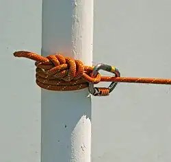
    A tensionless hitch around a post
    Names Tensionless Hitch, high-strength tie-off, No-Knot
    Category Hitch
    Efficiency 100%
    Related Round turn and two half-hitches, Pipe hitch, Klemheist knot, Tugboat hitch
    Releasing Non-jamming
    Typical use anchor knot
    Caveat The anchor diameter should be at least 8X the rope diameter.[1] Also, the hitch will not stay in place without a load.
    ABoK 2047[2]

    A Tensionless hitch is an anchor knot used for rappelling or rope rescue. Unlike most knots, the tensionless hitch retains a 100% efficiency rating,[3] meaning the strength of the knot is equal to the strength of the rope; it is not a significant stress riser.

    Tying

    The working end of a rope is prepared by tying a figure-eight loop, and then clipping a carabiner through that loop.

    The rope is then wrapped around a smooth pole, pipe, round beam or tree branch which has a diameter greater than the rope. The rope is typically wrapped 3 to 4 times around the anchor, without crossing. Finally, the working end is attached to the standing part with the carabiner.

    An overhand knot may be tied around the standing part before the final wrap around the anchor.[4]

    References

    1. “Tensionless Hitch”. Knots 3D. Nynix LLC. Retrieved 5 May 2016.
    2. Ashley, Clifford W. (1993) [1944], The Ashley Book of Knots, New York: Doubleday, p. 332, ISBN 0-385-04025-3
    3. Technical Rescue: Rope Rescue Accessed: 11/24/2013
    4. “ANCHORS AWAY: Learn How to Tie a High-Strength Tie-Off Anchor”. CMC Rescue. Retrieved 5 May 2016.

    External links


    This article is adapted from “Tensionless hitch” on Wikipedia, written by its contributors, and used under CC BY-SA 4.0. Text on this page is available under the same licence. Source snapshot: Wikipedia via Kiwix, 2026-07-20.

  • Double overhand noose

    Double overhand noose
    Double overhand noose
    Names Double overhand noose, Scaffold,[1][2] Poacher’s Knot[3]
    Category Hitch
    Efficiency High
    Related Noose, Double overhand knot, Double fisherman’s knot
    Releasing Jamming
    Typical use Bind a carabiner
    Caveat Difficult to untie
    ABoK #409, #1120, #1228

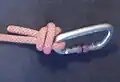
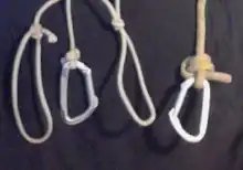
    The double overhand noose is a very secure hitch knot. It might be used by cavers and canyoneers to bind a cow tail or a foot loop to a carabiner.[4]

    Double overhand noose
    Double overhand noose binding carabiners.[a][b]

    Details

    A heavily tightened double overhand noose will jam. The bound object has to be removed before untying.

    As the double overhand knot, it neither slips nor turns around. However, a third round turn might be useful with some highly lubricious spectra/nylon ropes.[5]

    See also

    Notes

    1. The running end is stored in the bight.
    2. Foot loops tied with a zeppelin loop and an alpine butterfly knot.

    References

    1. Ashley, Clifford W.. The Ashley Book of Knots. Published by Faber and Faber, 1993 — #1120 — ISBN 9780571096596
    2. The complete guide to knots and knot tying — Geoffrey Budworth — p.37 — ISBN 0-7548-0422-4
    3. Ashley, Clifford W. (1944). The Ashley Book of Knots, Doubleday, p.65, #409. ISBN 0-385-04025-3
    4. Les longes en spéléologie et descente de canyon Archived March 31, 2012, at the Wayback Machine (in French)
    5. Tom Moyer, Paul Tusting, Chris Harmston,(2000) Comparative Testing of High Strength Cord

    This article is adapted from “Double overhand noose” on Wikipedia, written by its contributors, and used under CC BY-SA 4.0. Text on this page is available under the same licence. Source snapshot: Wikipedia via Kiwix, 2026-07-20.

  • Temperley–Lieb algebra

    In statistical mechanics, the Temperley–Lieb algebra is an algebra from which are built certain transfer matrices, invented by Neville Temperley and Elliott Lieb. It is also related to integrable models, knot theory and the braid groups, quantum groups and subfactors of von Neumann algebras.

    Structure

    Generators and relations

    Let R {\displaystyle R} {\displaystyle R} be a commutative ring and fix δ R {\displaystyle \delta \in R} {\displaystyle \delta \in R}. The Temperley–Lieb algebra T L n ( δ ) {\displaystyle TL_{n}(\delta )} {\displaystyle TL_{n}(\delta )} is the unital associative R {\displaystyle R} {\displaystyle R}-algebra generated by the elements e 1 , e 2 , , e n 1 {\displaystyle e_{1},e_{2},\ldots ,e_{n-1}} {\displaystyle e_{1},e_{2},\ldots ,e_{n-1}}, subject to the Jones relations:

    • e i 2 = δ e i {\displaystyle e_{i}^{2}=\delta e_{i}} {\displaystyle e_{i}^{2}=\delta e_{i}} for all 1 i n 1 {\displaystyle 1\leq i\leq n-1} {\displaystyle 1\leq i\leq n-1}
    • e i e i + 1 e i = e i {\displaystyle e_{i}e_{i+1}e_{i}=e_{i}} {\displaystyle e_{i}e_{i+1}e_{i}=e_{i}} for all 1 i n 2 {\displaystyle 1\leq i\leq n-2} {\displaystyle 1\leq i\leq n-2}
    • e i e i 1 e i = e i {\displaystyle e_{i}e_{i-1}e_{i}=e_{i}} {\displaystyle e_{i}e_{i-1}e_{i}=e_{i}} for all 2 i n 1 {\displaystyle 2\leq i\leq n-1} {\displaystyle 2\leq i\leq n-1}
    • e i e j = e j e i {\displaystyle e_{i}e_{j}=e_{j}e_{i}} {\displaystyle e_{i}e_{j}=e_{j}e_{i}} for all 1 i , j n 1 {\displaystyle 1\leq i,j\leq n-1} {\displaystyle 1\leq i,j\leq n-1} such that | i j | 1 {\displaystyle |i-j|\neq 1} {\displaystyle |i-j|\neq 1}

    Using these relations, any product of generators e i {\displaystyle e_{i}} {\displaystyle e_{i}} can be brought to Jones’ normal form:

    E = ( e i 1 e i 1 1 e j 1 ) ( e i 2 e i 2 1 e j 2 ) ( e i r e i r 1 e j r ) {\displaystyle E={\big (}e_{i_{1}}e_{i_{1}-1}\cdots e_{j_{1}}{\big )}{\big (}e_{i_{2}}e_{i_{2}-1}\cdots e_{j_{2}}{\big )}\cdots {\big (}e_{i_{r}}e_{i_{r}-1}\cdots e_{j_{r}}{\big )}} {\displaystyle E={\big (}e_{i_{1}}e_{i_{1}-1}\cdots e_{j_{1}}{\big )}{\big (}e_{i_{2}}e_{i_{2}-1}\cdots e_{j_{2}}{\big )}\cdots {\big (}e_{i_{r}}e_{i_{r}-1}\cdots e_{j_{r}}{\big )}}

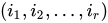
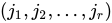
    where ( i 1 , i 2 , , i r ) {\displaystyle (i_{1},i_{2},\dots ,i_{r})} {\displaystyle (i_{1},i_{2},\dots ,i_{r})} and ( j 1 , j 2 , , j r ) {\displaystyle (j_{1},j_{2},\dots ,j_{r})} {\displaystyle (j_{1},j_{2},\dots ,j_{r})} are two strictly increasing sequences in { 1 , 2 , , n 1 } {\displaystyle \{1,2,\dots ,n-1\}} {\displaystyle \{1,2,\dots ,n-1\}}. Elements of this type form a basis of the Temperley-Lieb algebra.[1]

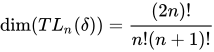
    The dimensions of Temperley-Lieb algebras are Catalan numbers:[2]

    dim ( T L n ( δ ) ) = ( 2 n ) ! n ! ( n + 1 ) ! {\displaystyle \dim(TL_{n}(\delta ))={\frac {(2n)!}{n!(n+1)!}}} {\displaystyle \dim(TL_{n}(\delta ))={\frac {(2n)!}{n!(n+1)!}}}

    The Temperley–Lieb algebra T L n ( δ ) {\displaystyle TL_{n}(\delta )} {\displaystyle TL_{n}(\delta )} is a subalgebra of the Brauer algebra B n ( δ ) {\displaystyle {\mathfrak {B}}_{n}(\delta )} {\displaystyle {\mathfrak {B}}_{n}(\delta )},[3] and therefore also of the partition algebra P n ( δ ) {\displaystyle P_{n}(\delta )} {\displaystyle P_{n}(\delta )}. The Temperley–Lieb algebra T L n ( δ ) {\displaystyle TL_{n}(\delta )} {\displaystyle TL_{n}(\delta )} is semisimple for δ C F n {\displaystyle \delta \in \mathbb {C} -F_{n}} {\displaystyle \delta \in \mathbb {C} -F_{n}} where F n {\displaystyle F_{n}} {\displaystyle F_{n}} is a known, finite set.[4] For a given n {\displaystyle n} {\displaystyle n}, all semisimple Temperley-Lieb algebras are isomorphic.[3]

    Diagram algebra

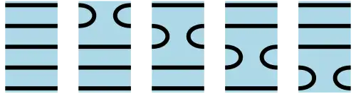
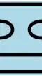
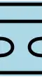
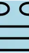
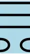
    T L n ( δ ) {\displaystyle TL_{n}(\delta )} {\displaystyle TL_{n}(\delta )} may be represented diagrammatically as the vector space over noncrossing pairings of 2 n {\displaystyle 2n} {\displaystyle 2n} points on two opposite sides of a rectangle with n points on each of the two sides.

    The identity element is the diagram in which each point is connected to the one directly across the rectangle from it. The generator e i {\displaystyle e_{i}} {\displaystyle e_{i}} is the diagram in which the i {\displaystyle i} {\displaystyle i}-th and ( i + 1 ) {\displaystyle (i+1)} {\displaystyle (i+1)}-th point on the left side are connected to each other, similarly the two points opposite to these on the right side, and all other points are connected to the point directly across the rectangle.

    The generators of T L 5 ( δ ) {\displaystyle TL_{5}(\delta )} {\displaystyle TL_{5}(\delta )} are:

    Generators of the Temperley–Lieb algebra 


        T
        
          L
          
            5
          
        
        (
        δ
        )
      
    
    {\displaystyle TL_{5}(\delta )}

    From left to right, the unit 1 and the generators e 1 {\displaystyle e_{1}} {\displaystyle e_{1}}, e 2 {\displaystyle e_{2}} {\displaystyle e_{2}}, e 3 {\displaystyle e_{3}} {\displaystyle e_{3}}, e 4 {\displaystyle e_{4}} {\displaystyle e_{4}}.

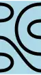
    Multiplication on basis elements can be performed by concatenation: placing two rectangles side by side, and replacing any closed loops by a factor δ {\displaystyle \delta } {\displaystyle \delta }, for example e 1 e 4 e 3 e 2 × e 2 e 4 e 3 = δ e 1 e 4 e 3 e 2 e 4 e 3 {\displaystyle e_{1}e_{4}e_{3}e_{2}\times e_{2}e_{4}e_{3}=\delta \,e_{1}e_{4}e_{3}e_{2}e_{4}e_{3}} {\displaystyle e_{1}e_{4}e_{3}e_{2}\times e_{2}e_{4}e_{3}=\delta \,e_{1}e_{4}e_{3}e_{2}e_{4}e_{3}}:

    Temperley–Lieb algebra × Temperley–Lieb algebra = Temperley–Lieb algebraTemperley–Lieb algebra = δ {\displaystyle \delta } {\displaystyle \delta } Temperley–Lieb algebra.

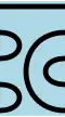
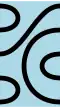
    The Jones relations can be seen graphically:

    Temperley–Lieb algebra Temperley–Lieb algebra = δ {\displaystyle \delta } {\displaystyle \delta } Temperley–Lieb algebra

    Temperley–Lieb algebra Temperley–Lieb algebra Temperley–Lieb algebra = Temperley–Lieb algebra

    Temperley–Lieb algebra Temperley–Lieb algebra = Temperley–Lieb algebra Temperley–Lieb algebra

    The five basis elements of T L 3 ( δ ) {\displaystyle TL_{3}(\delta )} {\displaystyle TL_{3}(\delta )} are the following:

    Basis of the Temperley–Lieb algebra 


        T
        
          L
          
            3
          
        
        (
        δ
        )
      
    
    {\displaystyle TL_{3}(\delta )}.

    From left to right, the unit 1, the generators e 2 {\displaystyle e_{2}} {\displaystyle e_{2}}, e 1 {\displaystyle e_{1}} {\displaystyle e_{1}}, and e 1 e 2 {\displaystyle e_{1}e_{2}} {\displaystyle e_{1}e_{2}}, e 2 e 1 {\displaystyle e_{2}e_{1}} {\displaystyle e_{2}e_{1}}.

    Representations

    Structure

    For δ {\displaystyle \delta } {\displaystyle \delta } such that T L n ( δ ) {\displaystyle TL_{n}(\delta )} {\displaystyle TL_{n}(\delta )} is semisimple, a complete set { W } {\displaystyle \{W_{\ell }\}} {\displaystyle \{W_{\ell }\}} of simple modules is parametrized by integers 0 n {\displaystyle 0\leq \ell \leq n} {\displaystyle 0\leq \ell \leq n} with n mod 2 {\displaystyle \ell \equiv n{\bmod {2}}} {\displaystyle \ell \equiv n{\bmod {2}}}. The dimension of a simple module is written in terms of binomial coefficients as[4]

    dim ( W ) = ( n n 2 ) ( n n 2 1 ) {\displaystyle \dim(W_{\ell })={\binom {n}{\frac {n-\ell }{2}}}-{\binom {n}{{\frac {n-\ell }{2}}-1}}} {\displaystyle \dim(W_{\ell })={\binom {n}{\frac {n-\ell }{2}}}-{\binom {n}{{\frac {n-\ell }{2}}-1}}}

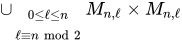
    A basis of the simple module W {\displaystyle W_{\ell }} {\displaystyle W_{\ell }} is the set M n , {\displaystyle M_{n,\ell }} {\displaystyle M_{n,\ell }} of monic noncrossing pairings from n {\displaystyle n} {\displaystyle n} points on the left to {\displaystyle \ell } {\displaystyle \ell } points on the right. (Monic means that each point on the right is connected to a point on the left.) There is a natural bijection between 0 n n mod 2 M n , × M n , {\displaystyle \cup _{\begin{array}{c}0\leq \ell \leq n\\\ell \equiv n{\bmod {2}}\end{array}}M_{n,\ell }\times M_{n,\ell }} {\displaystyle \cup _{\begin{array}{c}0\leq \ell \leq n\\\ell \equiv n{\bmod {2}}\end{array}}M_{n,\ell }\times M_{n,\ell }}, and the set of diagrams that generate T L n ( δ ) {\displaystyle TL_{n}(\delta )} {\displaystyle TL_{n}(\delta )}: any such diagram can be cut into two elements of M n , {\displaystyle M_{n,\ell }} {\displaystyle M_{n,\ell }} for some {\displaystyle \ell } {\displaystyle \ell }.

    Then T L n ( δ ) {\displaystyle TL_{n}(\delta )} {\displaystyle TL_{n}(\delta )} acts on W {\displaystyle W_{\ell }} {\displaystyle W_{\ell }} by diagram concatenation from the left.[3] (Concatenation can produce non-monic pairings, which have to be modded out.) The module W {\displaystyle W_{\ell }} {\displaystyle W_{\ell }} may be called a standard module or link module.[1]

    If δ = q + q 1 {\displaystyle \delta =q+q^{-1}} {\displaystyle \delta =q+q^{-1}} with q {\displaystyle q} {\displaystyle q} a root of unity, T L n ( δ ) {\displaystyle TL_{n}(\delta )} {\displaystyle TL_{n}(\delta )} may not be semisimple, and W {\displaystyle W_{\ell }} {\displaystyle W_{\ell }} may not be irreducible:

    W  reducible  j { 1 , 2 , , } ,   q 2 n 4 + 2 + 2 j = 1 {\displaystyle W_{\ell }{\text{ reducible }}\iff \exists j\in \{1,2,\dots ,\ell \},\ q^{2n-4\ell +2+2j}=1} {\displaystyle W_{\ell }{\text{ reducible }}\iff \exists j\in \{1,2,\dots ,\ell \},\ q^{2n-4\ell +2+2j}=1}

    If W {\displaystyle W_{\ell }} {\displaystyle W_{\ell }} is reducible, then its quotient by its maximal proper submodule is irreducible.[1]

    Branching rules from the Brauer algebra

    Simple modules of the Brauer algebra B n ( δ ) {\displaystyle {\mathfrak {B}}_{n}(\delta )} {\displaystyle {\mathfrak {B}}_{n}(\delta )} can be decomposed into simple modules of the Temperley-Lieb algebra. The decomposition is called a branching rule, and it is a direct sum with positive integer coefficients:

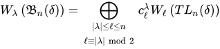
    W λ ( B n ( δ ) ) = | λ | n | λ | mod 2 c λ W ( T L n ( δ ) ) {\displaystyle W_{\lambda }\left({\mathfrak {B}}_{n}(\delta )\right)=\bigoplus _{\begin{array}{c}|\lambda |\leq \ell \leq n\\\ell \equiv |\lambda |{\bmod {2}}\end{array}}c_{\ell }^{\lambda }W_{\ell }\left(TL_{n}(\delta )\right)} {\displaystyle W_{\lambda }\left({\mathfrak {B}}_{n}(\delta )\right)=\bigoplus _{\begin{array}{c}|\lambda |\leq \ell \leq n\\\ell \equiv |\lambda |{\bmod {2}}\end{array}}c_{\ell }^{\lambda }W_{\ell }\left(TL_{n}(\delta )\right)}

    The coefficients c λ {\displaystyle c_{\ell }^{\lambda }} {\displaystyle c_{\ell }^{\lambda }} do not depend on n , δ {\displaystyle n,\delta } {\displaystyle n,\delta }, and are given by[4]

    c λ = f λ r = 0 | λ | 2 ( 1 ) r ( r r ) ( 2 r | λ | 2 r ) ( | λ | 2 r ) ! ! {\displaystyle c_{\ell }^{\lambda }=f^{\lambda }\sum _{r=0}^{\frac {\ell -|\lambda |}{2}}(-1)^{r}{\binom {\ell -r}{r}}{\binom {\ell -2r}{\ell -|\lambda |-2r}}(\ell -|\lambda |-2r)!!} {\displaystyle c_{\ell }^{\lambda }=f^{\lambda }\sum _{r=0}^{\frac {\ell -|\lambda |}{2}}(-1)^{r}{\binom {\ell -r}{r}}{\binom {\ell -2r}{\ell -|\lambda |-2r}}(\ell -|\lambda |-2r)!!}

    where f λ {\displaystyle f^{\lambda }} {\displaystyle f^{\lambda }} is the number of standard Young tableaux of shape λ {\displaystyle \lambda } {\displaystyle \lambda }, given by the hook length formula.

    Affine Temperley-Lieb algebra

    The affine Temperley-Lieb algebra a T L n ( δ ) {\displaystyle aTL_{n}(\delta )} {\displaystyle aTL_{n}(\delta )} is an infinite-dimensional algebra such that T L n ( δ ) a T L n ( δ ) {\displaystyle TL_{n}(\delta )\subset aTL_{n}(\delta )} {\displaystyle TL_{n}(\delta )\subset aTL_{n}(\delta )}. It is obtained by adding generators e n , τ , τ 1 {\displaystyle e_{n},\tau ,\tau ^{-1}} {\displaystyle e_{n},\tau ,\tau ^{-1}} such that[5]

    • τ e i = e i + 1 τ {\displaystyle \tau e_{i}=e_{i+1}\tau } {\displaystyle \tau e_{i}=e_{i+1}\tau } for all 1 i n {\displaystyle 1\leq i\leq n} {\displaystyle 1\leq i\leq n},
    • e 1 τ 2 = e 1 e 2 e n 1 {\displaystyle e_{1}\tau ^{2}=e_{1}e_{2}\cdots e_{n-1}} {\displaystyle e_{1}\tau ^{2}=e_{1}e_{2}\cdots e_{n-1}},
    • τ τ 1 = τ 1 τ = id {\displaystyle \tau \tau ^{-1}=\tau ^{-1}\tau ={\text{id}}} {\displaystyle \tau \tau ^{-1}=\tau ^{-1}\tau ={\text{id}}}.

    The indices are supposed to be periodic i.e. e n + 1 = e 1 , e n = e 0 {\displaystyle e_{n+1}=e_{1},e_{n}=e_{0}} {\displaystyle e_{n+1}=e_{1},e_{n}=e_{0}}, and the Temperley-Lieb relations are supposed to hold for all 1 i n {\displaystyle 1\leq i\leq n} {\displaystyle 1\leq i\leq n}. Then τ n {\displaystyle \tau ^{n}} {\displaystyle \tau ^{n}} is central. A finite-dimensional quotient of the algebra a T L n ( δ ) {\displaystyle aTL_{n}(\delta )} {\displaystyle aTL_{n}(\delta )}, sometimes called the unoriented Jones-Temperley-Lieb algebra,[6] is obtained by
    assuming τ n = id {\displaystyle \tau ^{n}={\text{id}}} {\displaystyle \tau ^{n}={\text{id}}}, and replacing non-contractible lines with the same factor δ {\displaystyle \delta } {\displaystyle \delta } as contractible lines (for example, in the case n = 4 {\displaystyle n=4} {\displaystyle n=4}, this implies e 1 e 3 e 2 e 4 e 1 e 3 = δ 2 e 1 e 3 {\displaystyle e_{1}e_{3}e_{2}e_{4}e_{1}e_{3}=\delta ^{2}e_{1}e_{3}} {\displaystyle e_{1}e_{3}e_{2}e_{4}e_{1}e_{3}=\delta ^{2}e_{1}e_{3}}).

    The diagram algebra for a T L n ( δ ) {\displaystyle aTL_{n}(\delta )} {\displaystyle aTL_{n}(\delta )} is deduced from the diagram algebra for T L n ( δ ) {\displaystyle TL_{n}(\delta )} {\displaystyle TL_{n}(\delta )} by turning rectangles into cylinders. The algebra a T L n ( δ ) {\displaystyle aTL_{n}(\delta )} {\displaystyle aTL_{n}(\delta )} is infinite-dimensional because lines can wind around the cylinder. If n {\displaystyle n} {\displaystyle n} is even, there can even exist closed winding lines, which are non-contractible.

    The Temperley-Lieb algebra is a quotient of the corresponding affine Temperley-Lieb algebra.[5]

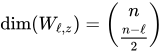
    The cell module W , z {\displaystyle W_{\ell ,z}} {\displaystyle W_{\ell ,z}} of a T L n ( δ ) {\displaystyle aTL_{n}(\delta )} {\displaystyle aTL_{n}(\delta )} is generated by the set of monic pairings from n {\displaystyle n} {\displaystyle n} points to {\displaystyle \ell } {\displaystyle \ell } points, just like the module W {\displaystyle W_{\ell }} {\displaystyle W_{\ell }} of T L n ( δ ) {\displaystyle TL_{n}(\delta )} {\displaystyle TL_{n}(\delta )}. However, the pairings are now on a cylinder, and the right-multiplication with τ {\displaystyle \tau } {\displaystyle \tau } is identified with z id {\displaystyle z\cdot {\text{id}}} {\displaystyle z\cdot {\text{id}}} for some z C {\displaystyle z\in \mathbb {C} ^{*}} {\displaystyle z\in \mathbb {C} ^{*}}. If = 0 {\displaystyle \ell =0} {\displaystyle \ell =0}, there is no right-multiplication by τ {\displaystyle \tau } {\displaystyle \tau }, and it is the addition of a non-contractible loop on the right which is identified with z + z 1 {\displaystyle z+z^{-1}} {\displaystyle z+z^{-1}}. Cell modules are finite-dimensional, with

    dim ( W , z ) = ( n n 2 ) {\displaystyle \dim(W_{\ell ,z})={\binom {n}{\frac {n-\ell }{2}}}} {\displaystyle \dim(W_{\ell ,z})={\binom {n}{\frac {n-\ell }{2}}}}

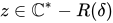
    The cell module W , z {\displaystyle W_{\ell ,z}} {\displaystyle W_{\ell ,z}} is irreducible for all z C R ( δ ) {\displaystyle z\in \mathbb {C} ^{*}-R(\delta )} {\displaystyle z\in \mathbb {C} ^{*}-R(\delta )}, where the set R ( δ ) {\displaystyle R(\delta )} {\displaystyle R(\delta )} is countable. For z R ( δ ) {\displaystyle z\in R(\delta )} {\displaystyle z\in R(\delta )}, W , z {\displaystyle W_{\ell ,z}} {\displaystyle W_{\ell ,z}} has an irreducible quotient. The irreducible cell modules and quotients thereof form a complete set of irreducible modules of a T L n ( δ ) {\displaystyle aTL_{n}(\delta )} {\displaystyle aTL_{n}(\delta )}.[5] Cell modules of the unoriented Jones-Temperley-Lieb algebra must obey z = 1 {\displaystyle z^{\ell }=1} {\displaystyle z^{\ell }=1} if 0 {\displaystyle \ell \neq 0} {\displaystyle \ell \neq 0}, and z + z 1 = δ {\displaystyle z+z^{-1}=\delta } {\displaystyle z+z^{-1}=\delta } if = 0 {\displaystyle \ell =0} {\displaystyle \ell =0}.

    Applications

    Temperley–Lieb Hamiltonian

    Consider an interaction-round-a-face model e.g. a square lattice model and let n {\displaystyle n} {\displaystyle n} be the number of sites on the lattice. Following Temperley and Lieb[7] we define the Temperley–Lieb Hamiltonian (the TL Hamiltonian) as
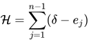
    H = j = 1 n 1 ( δ e j ) {\displaystyle {\mathcal {H}}=\sum _{j=1}^{n-1}(\delta -e_{j})} {\displaystyle {\mathcal {H}}=\sum _{j=1}^{n-1}(\delta -e_{j})}

    In what follows we consider the special case δ = 1 {\displaystyle \delta =1} {\displaystyle \delta =1}.

    We will firstly consider the case n = 3 {\displaystyle n=3} {\displaystyle n=3}. The TL Hamiltonian is H = 2 e 1 e 2 {\displaystyle {\mathcal {H}}=2-e_{1}-e_{2}} {\displaystyle {\mathcal {H}}=2-e_{1}-e_{2}}, namely

    H {\displaystyle {\mathcal {H}}} {\displaystyle {\mathcal {H}}} = 2 Temperley–Lieb algebraTemperley–Lieb algebraTemperley–Lieb algebra.

    We have two possible states,

    Temperley–Lieb algebra and Temperley–Lieb algebra.

    In acting by H {\displaystyle {\mathcal {H}}} {\displaystyle {\mathcal {H}}} on these states, we find

    H {\displaystyle {\mathcal {H}}} {\displaystyle {\mathcal {H}}} Temperley–Lieb algebra = 2 Temperley–Lieb algebraTemperley–Lieb algebraTemperley–Lieb algebraTemperley–Lieb algebraTemperley–Lieb algebraTemperley–Lieb algebra = Temperley–Lieb algebraTemperley–Lieb algebra,

    and

    H {\displaystyle {\mathcal {H}}} {\displaystyle {\mathcal {H}}} Temperley–Lieb algebra = 2 Temperley–Lieb algebraTemperley–Lieb algebraTemperley–Lieb algebraTemperley–Lieb algebraTemperley–Lieb algebraTemperley–Lieb algebra = – Temperley–Lieb algebra + Temperley–Lieb algebra.

    Writing H {\displaystyle {\mathcal {H}}} {\displaystyle {\mathcal {H}}} as a matrix in the basis of possible states we have,
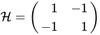
    H = ( 1 1 1 1 ) {\displaystyle {\mathcal {H}}=\left({\begin{array}{rr}1&-1\\-1&1\end{array}}\right)} {\displaystyle {\mathcal {H}}=\left({\begin{array}{rr}1&-1\\-1&1\end{array}}\right)}

    The eigenvector of H {\displaystyle {\mathcal {H}}} {\displaystyle {\mathcal {H}}} with the lowest eigenvalue is known as the ground state. In this case, the lowest eigenvalue λ 0 {\displaystyle \lambda _{0}} {\displaystyle \lambda _{0}} for H {\displaystyle {\mathcal {H}}} {\displaystyle {\mathcal {H}}} is λ 0 = 0 {\displaystyle \lambda _{0}=0} {\displaystyle \lambda _{0}=0}. The corresponding eigenvector is ψ 0 = ( 1 , 1 ) {\displaystyle \psi _{0}=(1,1)} {\displaystyle \psi _{0}=(1,1)}. As we vary the number of sites n {\displaystyle n} {\displaystyle n} we find the following table[8]

    n {\displaystyle n} {\displaystyle n} ψ 0 {\displaystyle \psi _{0}} {\displaystyle \psi _{0}} n {\displaystyle n} {\displaystyle n} ψ 0 {\displaystyle \psi _{0}} {\displaystyle \psi _{0}}
    2 (1) 3 (1, 1)
    4 (2, 1) 5 ( 3 3 , 1 2 ) {\displaystyle (3_{3},1_{2})} {\displaystyle (3_{3},1_{2})}
    6 ( 11 , 5 2 , 4 , 1 ) {\displaystyle (11,5_{2},4,1)} {\displaystyle (11,5_{2},4,1)} 7 ( 26 4 , 10 2 , 9 2 , 8 2 , 5 2 , 1 2 ) {\displaystyle (26_{4},10_{2},9_{2},8_{2},5_{2},1_{2})} {\displaystyle (26_{4},10_{2},9_{2},8_{2},5_{2},1_{2})}
    8 ( 170 , 75 2 , 71 , 56 2 , 50 , 30 , 14 4 , 6 , 1 ) {\displaystyle (170,75_{2},71,56_{2},50,30,14_{4},6,1)} {\displaystyle (170,75_{2},71,56_{2},50,30,14_{4},6,1)} 9 ( 646 , ) {\displaystyle (646,\ldots )} {\displaystyle (646,\ldots )}
    {\displaystyle \vdots } {\displaystyle \vdots } {\displaystyle \vdots } {\displaystyle \vdots } {\displaystyle \vdots } {\displaystyle \vdots } {\displaystyle \vdots } {\displaystyle \vdots }

    where we have used the notation m j = ( m , , m ) {\displaystyle m_{j}=(m,\ldots ,m)} {\displaystyle m_{j}=(m,\ldots ,m)} j {\displaystyle j} {\displaystyle j}-times e.g., 5 2 = ( 5 , 5 ) {\displaystyle 5_{2}=(5,5)} {\displaystyle 5_{2}=(5,5)}.

    An interesting observation is that the largest components of the ground state of H {\displaystyle {\mathcal {H}}} {\displaystyle {\mathcal {H}}} have a combinatorial enumeration as we vary the number of sites,[9] as was first observed by Murray Batchelor, Jan de Gier and Bernard Nienhuis.[8] Using the resources of the on-line encyclopedia of integer sequences, Batchelor et al. found, for an even numbers of sites

    1 , 2 , 11 , 170 , = j = 0 n 2 2 ( 3 j + 1 ) ( 2 j ) ! ( 6 j ) ! ( 4 j ) ! ( 4 j + 1 ) ! ( n = 2 , 4 , 6 , ) {\displaystyle 1,2,11,170,\ldots =\prod _{j=0}^{\frac {n-2}{2}}\left(3j+1\right){\frac {(2j)!(6j)!}{(4j)!(4j+1)!}}\qquad (n=2,4,6,\dots )} {\displaystyle 1,2,11,170,\ldots =\prod _{j=0}^{\frac {n-2}{2}}\left(3j+1\right){\frac {(2j)!(6j)!}{(4j)!(4j+1)!}}\qquad (n=2,4,6,\dots )}

    and for an odd numbers of sites

    1 , 3 , 26 , 646 , = j = 0 n 3 2 ( 3 j + 2 ) ( 2 j + 1 ) ! ( 6 j + 3 ) ! ( 4 j + 2 ) ! ( 4 j + 3 ) ! ( n = 3 , 5 , 7 , ) {\displaystyle 1,3,26,646,\ldots =\prod _{j=0}^{\frac {n-3}{2}}(3j+2){\frac {(2j+1)!(6j+3)!}{(4j+2)!(4j+3)!}}\qquad (n=3,5,7,\dots )} {\displaystyle 1,3,26,646,\ldots =\prod _{j=0}^{\frac {n-3}{2}}(3j+2){\frac {(2j+1)!(6j+3)!}{(4j+2)!(4j+3)!}}\qquad (n=3,5,7,\dots )}

    Surprisingly, these sequences corresponded to well known combinatorial objects. For n {\displaystyle n} {\displaystyle n} even, this (sequence A051255 in the OEIS) corresponds to cyclically symmetric transpose complement plane partitions and for n {\displaystyle n} {\displaystyle n} odd, (sequence A005156 in the OEIS), these correspond to alternating sign matrices symmetric about the vertical axis.
    XXZ spin chain

    References

    1. 1 2 3 Ridout, David; Saint-Aubin, Yvan (2012-04-20). “Standard Modules, Induction and the Temperley-Lieb Algebra”. arXiv:1204.4505v4 [math-ph].
    2. Kassel, Christian; Turaev, Vladimir (2008). “Braid Groups”. Graduate Texts in Mathematics. New York, NY: Springer New York. doi:10.1007/978-0-387-68548-9. ISBN 978-0-387-33841-5. ISSN 0072-5285.

    3. 1 2 3 Halverson, Tom; Jacobson, Theodore N. (2018-08-24). “Set-partition tableaux and representations of diagram algebras”. arXiv:1808.08118v2 [math.RT].
    4. 1 2 3 Benkart, Georgia; Moon, Dongho (2005-04-26), “Tensor product representations of Temperley-Lieb algebras and Chebyshev polynomials”, Representations of Algebras and Related Topics, Providence, Rhode Island: American Mathematical Society, pp. 57–80, doi:10.1090/fic/045/05, ISBN 9780821834152
    5. 1 2 3 Belletête, Jonathan; Saint-Aubin, Yvan (2018-02-10). “On the computation of fusion over the affine Temperley-Lieb algebra”. Nuclear Physics B. 937: 333–370. arXiv:1802.03575v1. Bibcode:2018NuPhB.937..333B. doi:10.1016/j.nuclphysb.2018.10.016. S2CID 119131017.
    6. Read, N.; Saleur, H. (2007-01-11). “Enlarged symmetry algebras of spin chains, loop models, and S-matrices”. Nuclear Physics B. 777 (3): 263–315. arXiv:cond-mat/0701259. Bibcode:2007NuPhB.777..263R. doi:10.1016/j.nuclphysb.2007.03.007. S2CID 119152756.
    7. Temperley, Neville; Lieb, Elliott (1971). “Relations between the ‘percolation’ and ‘colouring’ problem and other graph-theoretical problems associated with regular planar lattices: some exact results for the ‘percolation’ problem”. Proceedings of the Royal Society A: Mathematical, Physical and Engineering Sciences. 322 (1549): 251–280. Bibcode:1971RSPSA.322..251T. doi:10.1098/rspa.1971.0067. JSTOR 77727. MR 0498284. S2CID 122770421.
    8. 1 2 Batchelor, Murray; de Gier, Jan; Nienhuis, Bernard (2001). “The quantum symmetric X X Z {\displaystyle XXZ} {\displaystyle XXZ} chain at Δ = 1 / 2 {\displaystyle \Delta =-1/2} {\displaystyle \Delta =-1/2}, alternating-sign matrices and plane partitions”. Journal of Physics A. 34 (19): L265–L270. arXiv:cond-mat/0101385. doi:10.1088/0305-4470/34/19/101. MR 1836155. S2CID 118048447.
    9. de Gier, Jan (2005). “Loops, matchings and alternating-sign matrices”. Discrete Mathematics. 298 (1–3): 365–388. arXiv:math/0211285. doi:10.1016/j.disc.2003.11.060. MR 2163456. S2CID 2129159.

    Further reading


    This article is adapted from “Temperley–Lieb algebra” on Wikipedia, written by its contributors, and used under CC BY-SA 4.0. Text on this page is available under the same licence. Source snapshot: Wikipedia via Kiwix, 2026-07-20.

  • Double overhand knot

    Double overhand knot
    Double overhand knot
    Category Stopper
    Efficiency moderate
    Related overhand knot, surgeon’s knot, strangle knot, double fisherman’s knot
    ABoK #516
    A/B notation 51
    Double overhand knot
    Tying the knot
    Double overhand knot
    coil knot

    The double overhand knot[1] or barrel knot[2][3] is simply an extension of the regular overhand knot, made with one additional pass. The result is slightly larger and more difficult to untie. It forms the first part of the surgeon’s knot and both sides of a double fisherman’s knot. According to The Ashley Book of Knots, “A double overhand knot tied in a cat-o’-nine-tails is termed a blood knot.”[4]

    When weighted, it can be difficult to untie, especially when wet.[5][6]

    The strangle knot is a rearranged double overhand knot made around an object. It is sometimes used to secure items to posts.

    Instructions for tying

    1. Tie an overhand knot at the end of a rope but do not tighten the knot down.
    2. Pass the end of the line through the loop created by the first overhand knot.
    3. Tighten the knot down while sliding it into place at the end of the line. Be sure to leave some tail sticking out from the end of the knot.[7][8]

    Alternatively, the working end of the rope can be wrapped around the standing end twice, and then passed through both resulting loops.[2][3] Both methods result in the same knot, though the latter is easier to dress in the compact finished form.

    With either method, more loops can be included to make a longer multiple overhand knot (which is also known as a barrel knot or blood knot).[5][6]

    See also

    References

    1. Tilton, Buck (2008). Knots you need : step-by-step instructions for more than 100 of the best sailing, fishing, climbing, camping, and decorative knots. Bob Hede. Guilford, Conn.: Knack. ISBN 978-1-59921-395-8. OCLC 213765878.
    2. 1 2 “Barrel Knot”. 101Knots. 24 February 2018. Retrieved 2022-11-20.
    3. 1 2 Cunningham, Ryan (2020-03-10). “How To Tie A Barrel Knot – Survival World”. Survival World. Retrieved 2022-11-20.
    4. Ashley, Clifford W. (1944). The Ashley Book of Knots, p.82. Doubleday. ISBN 0-385-04025-3.
    5. 1 2 Bigon, Mario (1982). The Morrow guide to knots : for sailing, fishing, camping, climbing. Guido Regazzoni. New York: W. Morrow. p. 38. ISBN 0-688-01225-6. OCLC 8345653.
    6. 1 2 Owen, Peter (1993). Knots. Philadelphia, Pa.: Courage Books. p. 13. ISBN 1-56138-225-6. OCLC 28040872.
    7. “Double Overhand Stopper”. Animated Knots by Grog. Retrieved 2022-11-20.
    8. “Double Overhand Stopper Knot”. NetKnots.com. Archived from the original on 2016-10-18. Retrieved 2016-10-18.


    This article is adapted from “Double overhand knot” on Wikipedia, written by its contributors, and used under CC BY-SA 4.0. Text on this page is available under the same licence. Source snapshot: Wikipedia via Kiwix, 2026-07-20.

  • Taut-line hitch

    Taut-line hitch
    Taut-line hitch
    Names Taut-line hitch, Adjustable hitch, Rigger’s hitch, Tent-line hitch, Tent hitch
    Category Hitch
    Related Magnus hitch, Rolling hitch, Two half-hitches, Trucker’s hitch, Adjustable grip hitch
    ABoK #62, #1027, #1230, #1729, #1730, #1799, #1800, #1855, #1856, #1857, #1993

    The taut-line hitch is an adjustable loop knot for use on lines under tension. It is useful when the length of a line will need to be periodically adjusted in order to maintain tension. It is made by tying a rolling hitch around the standing part after passing around an anchor object. Tension is maintained by sliding the hitch to adjust the size of the loop, thus changing the effective length of the standing part without retying the knot.

    It is typically used for securing tent lines in outdoor activities involving camping, by arborists when climbing trees,[1] for tying down aircraft,[2] for creating adjustable moorings in tidal areas,[3] and to secure loads on vehicles. A versatile knot, the taut-line hitch was even used by astronauts during STS-82, the second Space Shuttle mission to repair the Hubble Space Telescope.[4]

    Naming

    Taut-line hitch
    Top, left to right: ABOK “Rolling hitch(1)”(#1734), “rolling hitch(2)”(#1735), “Magnus Hitch”(#1736). Bottom, the corresponding adjustable loop made using the hitch above it, left to right: “adjustable hitch”(#1800, #1856), “midshipman’s hitch”(#1855), “adjustable hitch” with the concluding hitch reversed.(#1857)

    The adjustable loop forms of the rolling hitch and Magnus hitch, in addition to being called either of those two names, have also come to be known variously as the taut-line hitch,[3] tent-line hitch,[3] rigger’s hitch,[3] adjustable hitch,[5] or midshipman’s hitch.[5] These knots are generally shown as being based on one of three underlying hitches: two variants of the rolling hitch (ABOK #1734 and #1735) and the Magnus hitch (#1736).

    These three closely related hitches have a long and muddled naming history that leads to ambiguity in the naming of their adjustable loop forms as well. The use of the Ashley reference numbers for these inconsistently named hitches can eliminate ambiguity when required. See the adjacent image for an illustration of these related knots.

    An early use of the taut-line hitch name is found in Howard W. Riley’s 1912 Knots, Hitches, and Splices, although it is shown in the rolling hitch form and suggested for use as a stopper.[6]

    Tying

    #1855

    Ashley uses the name midshipman’s hitch for this variation. Based on rolling hitch #1735, this version is considered the most secure but may be more difficult to adjust after being heavily loaded.

    Taut-line hitch
    1. Pass the working end around the anchor object. Bring it back alongside of the standing part and make a half-hitch around the standing part.
    2. Continue by passing the working end over the working part, around the standing part again and back through the loop formed in the first step. Make sure this second wrap tucks in between the first wrap and the working part of the line on the inside of the loop. This detail gives this version its additional security.
    3. Complete with a half-hitch outside the loop, made in the same direction as the first two wraps, as for a clove hitch.
    4. Dress by snugging the hitch firmly around the standing part. Load slowly and adjust as necessary.

    #1856

    Based on rolling hitch #1734, this version is the one most often seen named taut-line hitch, typically in non-nautical sources. It is the method currently taught by the Boy Scouts of America.[7] The earliest Boy Scout Handbook to include the taut-line hitch was the 5th edition, published in 1948.[8] However it illustrated #1855, the variant shown above.[9]

    Taut-line hitch
    1. Pass the working end around the anchor object. Bring it back alongside of the standing part and make a half-hitch around the standing part.
    2. Continue with another wrap inside the loop, effectively making a round turn around the standing part.
    3. Complete with a half-hitch outside the loop, made in the same direction as the first two wraps, as for a clove hitch.
    4. Dress by snugging the hitch firmly around the standing part. Load slowly and adjust as necessary.

    #1857

    Based on Magnus hitch #1736, this is exactly as above but with the final hitch in the opposite direction. It can be more tricky to snug-up, since both lines emerge from the same side of the hitch, but it has less tendency to twist under load.

    Taut-line hitch
    1. Pass the working end around the anchor object. Bring it back alongside of the standing part and make a half-hitch around the standing part.
    2. Continue with another wrap inside the loop, effectively making a round turn around the standing part.
    3. Complete with a half-hitch outside the loop made in the opposite direction than the first two wraps, as for a cow hitch.
    4. Dress by snugging the hitch firmly around the standing part. Load slowly and adjust as necessary.

    This is the form most commonly used for aircraft tie-down. One taut-line hitch is tied 15–30 cm from the aircraft and adjusted for tension, then a second taut-line hitch is tied 5–20 cm further from the aircraft and finished with a half-hitch. Wind-induced lift tends to pull the knot tighter, gust-induced oscillations tend to damp-out, and once the half hitch is undone, pushing the lower working rope up easily releases both hitches even amid icing.

    Adjusting

    Taut-line hitch
    Adjusting the guy-lines of a tent is a common use for the taut-line hitch.

    Once snug and set, the hitch can be adjusted as needed. To tighten the line with respect to a load attached to the standing part, the user can grasp the standing part with one hand inside of the loop and pull toward the anchor object. The hitch may be grasped with the other hand and as slack develops within the loop, the hitch slid away from the anchor object, taking up the slack and enlarging the loop. To loosen, the hitch may be slid toward the anchor object, making the loop smaller and lengthening the standing part.

    Security

    Although the three variations are similar, they do have distinct properties when put to use. Ashley[10] and others[3][11] suggest that #1855 is preferred as being more secure. Either #1856 or #1857 is also acceptable, especially if ease of adjustment is desired over security.[12][13] Ashley states #1857 has less tendency to twist.[5]

    These hitches may not hold fast under all conditions, and with lines made from particularly stiff or slick modern fibers (e.g. polypropylene) these hitches can be difficult to make hold at all. Sometimes they can be made more secure by using additional initial wraps and finishing half-hitches.[13]

    Friction hitches

    [14]
    These as a family are called Friction Hitches[1] or hold and release to slide hitches[15]

    The similar ABoK numbers are in ABoK’s unique “Chapter 22: Hitches to Masts, Rigging and Cable (Lengthwise Pull)[5] 1st paragraph reads: “To withstand a lengthwise pull without slipping is about the most that can be asked of a hitch. Great care must be exercised in tying the following series of knots, and the impossible must not be expected.”[5] A Friction Hitch is on a rope column that you are grabbing with “Lengthwise pull” force wise in this chapter.[5] Not at the best (right) angle to host mount the rest of the book speaks of and shows for working hitches and thus chapter title and preface states. And so, the Friction Hitches are contained in this chapter on the errant pull angle stated as “Lengthwise Pull”.[5] Book shows a ‘linear’ Half Hitch to precede a Timber Hitch (that shows should pull at right angle to spar) so can pull lengthwise in ABoK#”1733. The timber hitch and half hitch Killick hitch perhaps best demonstrates the directional force effect as he shows it as the first knot in the chapter right after the previous discussion as context .[5] After showing the Half-Hitch preceding as only conversion for the direction adds: “The knot appears to be universal and invariable”! [5]

    See also

    References

    1. 1 2 Adams, Mark (April 2005), “Son of a Hitch: A Genealogy of Arborists’ Climbing Hitches” (PDF), Arborist News, International Society of Arboriculture
    2. Pardo, Jeff (October 2004), “Tying the Knot: Know the ropes so your aircraft won’t be gone with the wind”, Flight Training, Airplane Owners and Pilots Association
    3. 1 2 3 4 5 Toss, Brion (1998), The Complete Rigger’s Apprentice, Camden: International Marine, pp. 54–55
    4. Nugent, Tom (1997). “Blanketing the Hubble”. University of Delaware Messenger. 6 (3).
    5. 1 2 3 4 5 6 7 8 9 Ashley, Clifford W. (1944), The Ashley Book of Knots, New York: Doubleday, p. 304
    6. Riley, Howard W. (January 1912). “Knots, Hitches, and Splices”. The Cornell Reading-Courses. Rural Engineering Series No. 1. 1 (8). Ithaca, NY: New York State College of Agriculture at Cornell University: 1425. Retrieved 2011-11-26. As not collected in Documents of the Assembly of the State of New York, 136th Session, 1913, Vol. 19, No. 29, Part 5.
    7. Boy Scouts of America (2009), The Boy Scout Handbook (12th ed.), Irving: BSA, p. 385
    8. Snowden, Jeff (2009), The Boy Scout Handbook 1910-Today (4th ed.), Troop 97 BSA
    9. Boy Scouts of America (1949), Handbook for Boys (5th ed.), BSA, pp. 94–95
    10. Ashley(1944), p. 298
    11. Trower, Nola (1995), Helmsman Guides: Knots and Ropework, Wiltshire: Helmsman Books, pp. 31–32
    12. Ashley(1944), p. 296
    13. 1 2 Toss, Brion (1990), Chapman’s Nautical Guides: Knots, New York: Hearst Marine Books, pp. 30–32
    14. Bavaresco, Paolo (2002). “Ropes and Friction Hitches used in Tree Climbing Operations” (PDF). Professional Association of Climbing Instructors PACI.com.
    15. Adams, Mark (October 2004). “Climber’s Corner an Overview of Climbing Hitches” (PDF). treebuzz.com.

    This article is adapted from “Taut-line hitch” on Wikipedia, written by its contributors, and used under CC BY-SA 4.0. Text on this page is available under the same licence. Source snapshot: Wikipedia via Kiwix, 2026-07-20.

  • Double figure-eight loop

    Double figure-eight loop
    Double figure-eight loop
    Names Double figure-eight loop, double Flemish loop, bunny ears
    Category Loop
    Related Figure-eight loop
    Typical use climbing, equalizing anchors
    ABoK #1085

    A double figure-eight loop, (also known as a bunny ears, or a dog eared loop) is a type of knot that forms two parallel loops, and resembles the figure-eight loop.[1]

    It is frequently used in climbing and caving as an easily untie-able knot that is capable of being attached to two bolts and equalised.[2]

    A variation of this knot exists, known as the double figure-eight follow through that creates another loop below the bulk of the knot, a feature that is useful for clipping safety ropes into.[3]

    References

    1. Ashley, Clifford W. (1944), The Ashley Book of Knots, New York: Doubleday, p. 197, ISBN 978-0-385-04025-9 {{citation}}: ISBN / Date incompatibility (help)
    2. “Bunny Ears: The Best Multi-pitch Climbing Knot You’ve Never Heard of”. Retrieved 2015-04-24.
    3. “Double Figure-8”. www.utgrotto.org. Retrieved 2015-04-24.

    External links


    This article is adapted from “Double figure-eight loop” on Wikipedia, written by its contributors, and used under CC BY-SA 4.0. Text on this page is available under the same licence. Source snapshot: Wikipedia via Kiwix, 2026-07-20.

  • Double bowline

    Double bowline
    Double bowline
    Names Double bowline, round turn bowline, double-knotted bowline
    Category Loop
    Efficiency 70-75%
    Related Bowline, water bowline, double sheet bend, bowline on a bight
    Typical use climbing
    ABoK #1013

    A double bowline (or round turn bowline) is a type of loop knot. Instead of the single turn of the regular bowline, the double bowline uses a round turn. This forms a more secure loop than a standard bowline.[1]

    Naming

    Though called “double bowline” by Clifford Ashley, this name is also reasonably descriptive of a different knot: the bowline on a bight. Because of this ambiguity
    some sources differentiate by using one of the alternate names above. And at least one other source uses the name “double bowline” for a mid-line loop knot made by tying a basic bowline with a bight of rope instead of the end.[2]

    Tying

    First, learn to tie the bowline by laying the working end on the standing part and twisting to form a loop (the “hole” that the rabbit comes out of). Wrap the loop once more around the working end. Then pass the working end behind the standing part and back down through the double loop.

    Uses

    The double bowline is one of the typical tie-in knots used in climbing, along with the figure eight follow through[3][4] and the Yosemite bowline.[5] The advantage of the double bowline over the figure 8 is that it is easier to untie after being weighted in a fall,[3][4] and so is used by sport climbers who take multiple lead falls and then have trouble untying their figure eights.[3][4] The disadvantages of the double bowline are that it is less secure than a figure eight knot, takes longer to tie, and is not as easy to check.[3][4] Unlike the figure eight, there are many variations of the bowline, with ambiguous names, and some are not safe for climbing.[6][7][8][9]

    The bowline on a bight, when re-threaded instead of being tied on a bight, can also be used for tying into a climbing harness and provides more strength and security than the double bowline.

    See also

    References

    1. Ashley, Clifford W (1944). The Ashley Book of Knots. New York: Doubleday. p. 186. ISBN 978-0-385-04025-9. OCLC 156951323. {{cite book}}: ISBN / Date incompatibility (help)
    2. Cox, Steven M.; Fulsaas, Kris, eds. (2003). Mountaineering: The Freedom of the Hills (7th ed.). The Mountaineers Books. p. 119. ISBN 978-0-89886-827-2.
    3. 1 2 3 4 Luebben, Craig (2004). Rock Climbing: Mastering Basic Skills. Seattle, WA: Mountaineers Books. p. 301. ISBN 978-0-89886-743-5.
    4. 1 2 3 4 Green, Stewart M; Ian, Spencer-Green; Mark, Doolittle (2010). Knack Rock Climbing: A Beginner’s Guide: From the Gym to the Rocks. Guilford, Connecticut: Globe Pequot. p. 256. ISBN 978-1-59921-852-6.
    5. Kidd, Timothy W.; Hazelrigs, Jennifer (2009). Rock Climbing. Human Kinetics. pp. 136. ISBN 9781450409001. Retrieved 12 October 2014.
    6. Heise-Flecken, Detlef; Flecken, Gabi (2016-03-28). Rock Climbing: Technique | Equipment | Safety – With an Introduction to Indoor Climbing. Meyer & Meyer Verlag. p. 20. ISBN 9781782550358. double bowline is more complicated than the Figure Eight and partner checks are harder to verify. … single bowline is not safe while the double bowline is difficult to tie but is easier to undo after taking strain
    7. “Incident: Climber’s Bowline Came Untied While Climbing at Rifle”. Mountain Project. Retrieved 2018-07-14. there are many versions of the bowline, some of which are unsafe for climbing … Bowline on a Bight, Retraced Through Harness w/ Yosemite Finish … is the safest option
    8. Rock Climbing. Human Kinetics. 2009. ISBN 9781450409001. Because this knot unties so easily, sometimes even by simply rubbing against your body
    9. Tilton, Buck (2008-09-02). Knack Knots You Need: Step-by-Step instructions for More Than 100 of the Best Sailing, Fishing, Climbing, Camping and Decorative Knots. Rowman & Littlefield. ISBN 9781599217598. A knot that can be shaken loose to spill of its own accord, such as the bowline … is an insecure knot.

    External links


    This article is adapted from “Double bowline” on Wikipedia, written by its contributors, and used under CC BY-SA 4.0. Text on this page is available under the same licence. Source snapshot: Wikipedia via Kiwix, 2026-07-20.