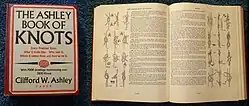
Category: Knots

  • Timber hitch

    Timber hitch
    Timber hitch
    Names Timber hitch, Fig.8 Timber Hitch, Bowyer’s Knot, Lumberman’s Knot, Countryman’s Knot
    Category Hitch
    Related Killick hitch
    Releasing Non-jamming
    ABoK #1668,#195, #479, #1665, #2161
    Instructions

    The timber hitch is a knot used to attach a single length of rope to a cylindrical object. Secure while tension is maintained, it is easily untied even after heavy loading.[1][2][3]

    The timber hitch is a very old knot. It is first known to have been mentioned in a nautical source c. 1625[4] and illustrated in 1762.[1]

    Usage

    As the name suggests, this knot is often used by lumbermen and arborists for attaching ropes or chains to tree trunks, branches, and logs.[3][5] For stability when towing or lowering long items, the addition of a half-hitch in front of the timber hitch creates a timber hitch and a half hitch,[6] or known as a killick hitch[2] when at sea.[7] A killick is “a small anchor or weight for mooring a boat, sometimes consisting of a stone secured by pieces of wood”.[8] This can also prevent the timber hitch from rolling.[3] The timber hitch is one of the few knots that can easily be tied in a chain, leading to its use in applications where ropes lack the necessary strength and would break under the same amount of tension.
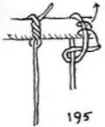
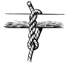
    Timber hitch

    The Timber Hitch is very convenient for hoisting boards and timbers, as it cannot jam and may be instantly loosened. If timber is to be hoisted on end the Timber Hitch is made with the end of the rope below the center of the timber and then a Half Hitch is added in the standing part at the upper end of the timber.

    Clifford W. Ashley, The Ashley Book of Knots, Entry 195.

    This knot is also known as the Bowyer’s Knot, as it is used to attach the lower end of the bowstring to the bottom limb on an English longbow.[9]

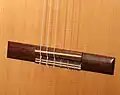
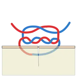
    The hitch is also one of the methods used to connect ukulele[10] and classical guitar[11][12] strings to the bridge of the instruments.

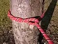
    • Timber hitch on a tree trunk.
      Timber hitch on a tree trunk.
    • Timber hitches on the bridge of a classical guitar
      Timber hitches on the bridge of a classical guitar

    Tying

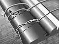
    To make the knot, pass the rope completely around the object. Pass the running end around the standing part, then through the loop just formed. Make three or more turns (or twists) around the working part. Pull on the standing part to tighten around the object.

    A common error in tying can be avoided by assuring that the turns are made in the working part around itself.[13] When making the hitch in laid rope, the turns should be made with the lay of the rope, that is, in the same direction as the twist of the rope.[1][2]

    • Timber hitch step by step. Three turns are shown.
      Timber hitch step by step. Three turns are shown.
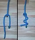
    • Tying technique for stringed instruments
      Tying technique for stringed instruments

    Security

    Although The Ashley Book of Knots states that “three tucks or turns are ample”,[1] this work was written prior to the wide use of synthetic fiber cordage. Later sources suggest five or more turns may be required for full security in modern synthetic ropes.[3][14]

    ABoK Context
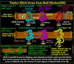
    Comparison of 3 types of Half Hitches, and then Timber Hitches, including Killik conversion for errant angle of pull.
    Comparison of 3 types of Half Hitches, and then Timber Hitches, including Killik conversion for errant angle of pull.

    The Timber Hitches list almost immediately in “CHAPTER 21: HITCHES TO SPAR AND RAIL (RIGHT-ANGLE PULL)”, only preceded there by 3 Half Hitch base forms. The context begins with typical Half Hitch#1662 as worst security/nip warnings warning with Skull/Crossbones, but a base structure to build on. Then shows the most security at top nip/opposing the linear load pull position as a safer Half Hitch form#1663 awarding Anchor icon if constant pull. Then introduces Timber Hitch #1665 concept from extension of worst nip Half Hitch tail#1662 . #1666 then shows Fig.8 concept as upgrade to Half Hitch#1662 and shows the nip position pushed to halfway between normal and top nip Half Hitch. Also adds a geometric consideration of:”particularly if the encompassed object is small.” of even higher nip. #1668 then shows the Fig.8 Timber Hitch with nip more to side and not bottom as improvement.[1]

    Next trick is in #1669 Fig.8 Hitch with Round Turn. Where the Round Turn is around the Standing Part and Fig.8 portion actually pictured as fig.8 Timber Hitch and so adds that the “Round Turn on the Standing Part adds materially to the strength of the knot.”[1]

    Next chapter is “CHAPTER 22: HITCHES TO MASTS, RIGGING, AND CABLE (LENGTHWISE PULL) To withstand a lengthwise pull without slipping is about the most that can be asked of a hitch. Great care must be exercised in tying the following series of knots, and the impossible must not be expected” that starts off with a Timber Hitch preceded by ‘lengthwise’ Half Hitch form to convert Timber from “RIGHT-ANGLE PULL” to “LENGTHWISE PULL” usage in the back to back chapters.[1]

    See also

    References

    1. 1 2 3 4 5 6 7 Ashley, Clifford W. (1944), The Ashley Book of Knots, New York: Doubleday, p. 290
    2. 1 2 3 Day, Cyrus Lawrence (1986), The Art of Knotting and Splicing (4th ed.), Annapolis: Naval Institute Press, pp. 94–95
    3. 1 2 3 4 Jepson, Jeff (2000), The Tree Climber’s Companion (2nd ed.), Minneapolis: Beaver Tree Publishing, p. 78
    4. Anderson, R.C.; Salisbury, W., eds. (1958), A Treatise on Rigging c. 1625, Occasional Publications No. 6, London: The Society for Nautical Research, p. 51, The Truss is fastened to the middle of the mayne yearde betwene the Parell with a tymber hitch and from thence goes through a blocke fastened to the mayne mast close to the middle decke and so to the Capstone when you will use him.
    5. Ashley (1944), p. 77
    6. Blandford, Percy (1965), Knots and Splices, New York, New York, USA: Arco Publishing Company, Inc, p. 23
    7. Blandford, Percy (1965), Knots and Splices, New York, New York, USA: Arco Publishing Company, Inc, p. 32
    8. “Killick”.
    9. Bickerstaffe, Pip (2010). “Tying the Bowyers Knot”. Grand Affairs Group. Archived from the original on 2012-04-26. Retrieved 2012-01-02.
    10. Wood, Alistair (2011), Ukulele For Dummies, Chichester, England: John Wiley & Sons, pp. 269–271
    11. Cumpiano, William R.; Natelson, Jonathan D. (1997), Guitarmaking, Tradition and Technology, San Francisco: Chronicle Books, pp. 368–369
    12. Pinksterboer, Hugo (2001), Tipbook Acoustic Guitar, Netherlands: The Tipbook Company, pp. 66–69
    13. Asher, Harry (1989), The Alternative Knot Book, London: Nautical Books, p. 32, ISBN 0-7136-5950-5
    14. Budworth, Geoffrey (1997), The Complete Book of Knots, New York, New York: Lyons & Burford, p. 47

    External links


    This article is adapted from “Timber hitch” on Wikipedia, written by its contributors, and used under CC BY-SA 4.0. Text on this page is available under the same licence. Source snapshot: Wikipedia via Kiwix, 2026-07-20.
  • Fairy-lock

    Fairy-lock
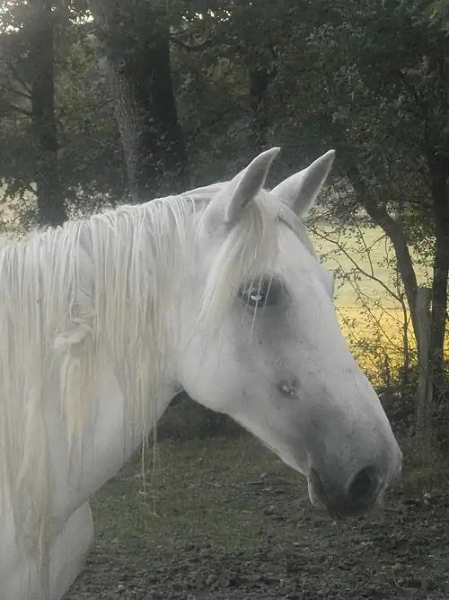
    A fairy-lock in the mane of a horse.

    In folklore, fairy-locks (or elflocks) are the result of fairies tangling and knotting the hairs of sleeping children and the manes of beasts as the fairies play in and out of their hair at night.[1]

    English tradition

    The concept is first attested in English in Shakespeare’s Romeo and Juliet in Mercutio’s speech of the many exploits of Queen Mab, where he seems to imply the locks are only unlucky if combed out:

    “She is the fairies’ midwife, and she comes
    In shape no bigger than an agate stone…….
    That plaits the manes of horses in the night
    And bakes the elflocks in foul sluttish hairs,
    Which once untangled, much misfortune bodes.”

    Therefore, the appellation of elf lock or fairy lock could be attributed to any various tangles and knots of unknown origins appearing in the manes of beasts or hair of sleeping children.

    It can also refer to tangles of elflocks or fairy-locks in human hair. In King Lear, when Edgar impersonates a madman, “elf all my hair in knots.”[2] (Lear, ii. 3.) What Edgar has done, simply put, is made a mess of his hair.

    See also Jane Eyre, Ch. XIX; Jane’s description of Rochester disguised as a gypsy: “… elf-locks bristled out from beneath a white band …”

    German tradition

    German counterparts of the “elf-lock” are Alpzopf, Drutenzopf, Wichtelzopf, Weichelzopf, Mahrenlocke, Elfklatte, etc. (where alp, drude, mare, and wight are given as the beings responsible). Grimm, who compiled the list, also remarked on the similarity to Frau Holle, who entangled people’s hair and herself had matted hair.[3] The use of the word elf seems to have declined steadily in English, becoming a rural dialect term, before being revived by translations of fairy tales in the nineteenth century and fantasy fiction in the twentieth.

    French tradition

    Fairy-locks are ascribed in French traditions to the lutin.[4]

    Eastern European tradition

    In Poland and nearby countries, witches and evil spirits were often blamed for Polish plait. This can be, however, a serious medical condition or an intentional hairstyle.

    References

    1. Batt, Tanya Robyn; Gail Newey (2002). A child’s book of faeries. Cambridge, Massachusetts: Barefoot Books. ISBN 1841489549.
    2. Shakespeare’s “Lear”.
    3. (Stallybrass tr.) Grimm 1883, vol. 2, p. 464
    4. Gary R. Butler, ‘The Lutin Tradition in French-Newfoundland Culture: Discourse and Belief’, in The Good People: New Fairylore Essays, ed. by Peter Narváez, Garland Reference Library of the Humanities, 1376 (New York: Garland, 1991), pp. 5–21.

    Works cited


    This article is adapted from “Fairy-lock” on Wikipedia, written by its contributors, and used under CC BY-SA 4.0. Text on this page is available under the same licence. Source snapshot: Wikipedia via Kiwix, 2026-07-20.

  • Thurston–Bennequin number

    In the mathematical theory of knots, the Thurston–Bennequin number, or Bennequin number, is an invariant associated with a Legendrian knot in a three dimensional contact manifold. It is named after William Thurston and Daniel Bennequin. The Thurston-Bennequin number measures the “twisting of the contact structure around the knot”.[1] Together with the rotation number, they are often referred as the “classical” invariants of Legendrian knots.

    The Thurston-Bennequin number of a Legendrian knot K {\displaystyle K} {\displaystyle K} is usually denoted by t b ( K ) {\displaystyle \mathrm {tb} (K)} {\displaystyle \mathrm {tb} (K)}. The maximal Thurston–Bennequin number, t b ¯ ( K ) {\displaystyle {\overline {\mathrm {tb} }}(K)} {\displaystyle {\overline {\mathrm {tb} }}(K)}, over all Legendrian representatives of a knot in R 3 {\displaystyle \mathbb {R} ^{3}} {\displaystyle \mathbb {R} ^{3}} is a topological knot invariant.[2]

    Definition and properties

    Let K {\displaystyle K} {\displaystyle K} be a null-homologous oriented Legendrian knot in a co-oriented three-dimensional contact manifold ( M 3 , ξ ) {\displaystyle (M^{3},\xi )} {\displaystyle (M^{3},\xi )} and fix a Seifert surface Σ {\displaystyle \Sigma } {\displaystyle \Sigma } to K {\displaystyle K} {\displaystyle K}, that is an embedded connected, compact, orientable surface with boundary Σ = K {\displaystyle \partial \Sigma =K} {\displaystyle \partial \Sigma =K}. The Thurston-Bennequin number of K {\displaystyle K} {\displaystyle K} relative to Σ {\displaystyle \Sigma } {\displaystyle \Sigma } is the defined as the signed intersection number of the contact plane field ξ {\displaystyle \xi } {\displaystyle \xi } with Σ {\displaystyle \Sigma } {\displaystyle \Sigma }.[3]

    Let K {\displaystyle K’} {\displaystyle K'} be a small push-off of K {\displaystyle K} {\displaystyle K} obtained by pushing along a vector field v {\displaystyle v} {\displaystyle v} transverse to ξ {\displaystyle \xi } {\displaystyle \xi }. The Thurston-Bennequin number can also be defined as l k ( K , K ) {\displaystyle \mathrm {lk} (K,K’)} {\displaystyle \mathrm {lk} (K,K')}, where l k {\displaystyle \mathrm {lk} } {\displaystyle \mathrm {lk} } denotes the linking number.[3]

    The Euclidean case

    We consider the case where ( M , ξ ) = ( R 3 , ξ s t d ) {\displaystyle (M,\xi )=(\mathbb {R} ^{3},\xi _{\mathrm {std} })} {\displaystyle (M,\xi )=(\mathbb {R} ^{3},\xi _{\mathrm {std} })} is the standard contact structure on R 3 {\displaystyle \mathbb {R} ^{3}} {\displaystyle \mathbb {R} ^{3}}. If we denote ( x , y , z ) {\displaystyle (x,y,z)} {\displaystyle (x,y,z)} the coordinates in R 3 {\displaystyle \mathbb {R} ^{3}} {\displaystyle \mathbb {R} ^{3}}, the contact structure ξ s t d {\displaystyle \xi _{\mathrm {std} }} {\displaystyle \xi _{\mathrm {std} }} is the kernel of the one-form d z y d x {\displaystyle dz-ydx} {\displaystyle dz-ydx}. The applications Π : R 3 R 2 , ( x , y , z ) ( x , z ) {\displaystyle \Pi \colon \mathbb {R} ^{3}\to \mathbb {R} ^{2},(x,y,z)\mapsto (x,z)} {\displaystyle \Pi \colon \mathbb {R} ^{3}\to \mathbb {R} ^{2},(x,y,z)\mapsto (x,z)} and π L : R 3 R 2 , ( x , y , z ) ( x , y ) {\displaystyle \pi _{L}\colon \mathbb {R} ^{3}\to \mathbb {R} ^{2},(x,y,z)\mapsto (x,y)} {\displaystyle \pi _{L}\colon \mathbb {R} ^{3}\to \mathbb {R} ^{2},(x,y,z)\mapsto (x,y)} denote respectively the front projection and the Lagrangian projection. The Thurston-Bennequin number can be computed easily from its front and Lagrangian projections.

    Lagrangian projection description

    The Thurston-Bennequin number of a Legendrian knot K R 3 {\displaystyle K\subset \mathbb {R} ^{3}} {\displaystyle K\subset \mathbb {R} ^{3}} is the writhe of its Lagrangian projection π L ( K ) {\displaystyle \pi _{L}(K)} {\displaystyle \pi _{L}(K)}.

    Front projection description

    For a Legendrian knot K R 3 {\displaystyle K\subset \mathbb {R} ^{3}} {\displaystyle K\subset \mathbb {R} ^{3}}, its front projection Π ( K ) R 2 {\displaystyle \Pi (K)\subset \mathbb {R} ^{2}} {\displaystyle \Pi (K)\subset \mathbb {R} ^{2}} is called its front diagram. The front diagram of a Legendrian knot does not have vertical tangencies, however cusps can appear. Generically, the front diagram of a knot as no tangency point, no triple intersection and standard cusp singularities. In this case the Thurston-Bennequin number is

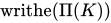
    t b ( K ) = writhe ( Π ( K ) ) 1 2 ( # number of cusps ) , {\displaystyle \mathrm {tb} (K)={\textrm {writhe}}(\Pi (K))-{\dfrac {1}{2}}{\big (}\#{\text{number of cusps}}{\big )},} {\displaystyle \mathrm {tb} (K)={\textrm {writhe}}(\Pi (K))-{\dfrac {1}{2}}{\big (}\#{\text{number of cusps}}{\big )},}

    where writhe ( Π ( K ) ) {\displaystyle {\textrm {writhe}}(\Pi (K))} {\displaystyle {\textrm {writhe}}(\Pi (K))} denotes the writhe of the front diagram.[1]

    The invariant can also be computed using a grid diagram corresponding to a particular Legendrian representative of a knot.[4][5] In this setting, the number can be computed as the writhe of the diagram minus the number of ‘northwest’ corners.

    Thurston–Bennequin number
    A grid diagram of the knot 8 20 {\displaystyle 8_{20}} {\displaystyle 8_{20}} and an associated Legendrian representative of it.

    By smoothing the ‘northeast’ and ‘southwest’ corners and rotating the diagram and switching all crossings, one can convert a grid diagram into the associated Legendrian knot.

    The Bennequin inequality

    In his thesis [1], Daniel Bennequin proved an inequality involving the Thurston-Bennequin number. He proved that for all Legendrian knot K {\displaystyle K} {\displaystyle K} in the standard contact R 3 {\displaystyle \mathbb {R} ^{3}} {\displaystyle \mathbb {R} ^{3}} the following inequality is true:

    t b ( K ) + | rot ( K ) | χ ( Σ ) , {\displaystyle \mathrm {tb} (K)+\vert {\textrm {rot}}(K)\vert \leq -\chi (\Sigma ),} {\displaystyle \mathrm {tb} (K)+\vert {\textrm {rot}}(K)\vert \leq -\chi (\Sigma ),}

    where χ ( Σ ) {\displaystyle \chi (\Sigma )} {\displaystyle \chi (\Sigma )} denotes the Euler characteristic of a Seifert surface Σ {\displaystyle \Sigma } {\displaystyle \Sigma } of K {\displaystyle K} {\displaystyle K} and rot ( K ) {\displaystyle {\textrm {rot}}(K)} {\displaystyle {\textrm {rot}}(K)} denotes the rotation number of K {\displaystyle K} {\displaystyle K}.

    In particular, the maximal Thurston-Bennequin number gives a lower bound on the genus of a topological knot.

    References

    1. 1 2 3 “Entrelacements et équations de Pfaff”. Astérisque. 107/108: 87–161. 1983. (Bennequin’s doctoral dissertation)
    2. Ng, Lenhard (2012). “On arc index and maximal thurston–bennequin number”. Journal of Knot Theory and Its Ramifications. 21 (04): 1250031. arXiv:math/0612356. doi:10.1142/S0218216511009820. ISSN 0218-2165.
    3. 1 2 Geiges, Hansjörg (2008). An introduction to contact topology; Volume 109 of Cambridge studies in advanced mathematics. Cambridge University Press. p. 94. ISBN 978-0-521-86585-2.
    4. Ozsváth, Peter S.; Stipsicz, András I.; Szabó, Zoltán (2015). Grid Homology for Knots and Links. American Mathematical Society. pp. 220–221. ISBN 978-1-4704-3442-7.
    5. Dynnikov, I.; Prasolov, M. (2013). “Bypasses for rectangular diagrams. A proof of the Jones conjecture and related questions”. Transactions of the Moscow Mathematical Society. 74: 97–144. arXiv:1206.0898. doi:10.1090/S0077-1554-2014-00210-7. ISSN 0077-1554.


    This article is adapted from “Thurston–Bennequin number” on Wikipedia, written by its contributors, and used under CC BY-SA 4.0. Text on this page is available under the same licence. Source snapshot: Wikipedia via Kiwix, 2026-07-20.

  • Eskimo bowline

    Eskimo Bowline
    Eskimo bowline
    Names Eskimo Bowline, Sitka Loop, Anti-bowline, Cossack knot
    Category Loop
    Origin Ancient
    Related Kalmyk loop, Bowline, Cowboy bowline, Sheet bend
    Releasing Non-jamming
    Typical use Placing a loop in the end of a rope

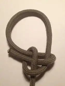
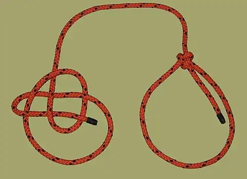
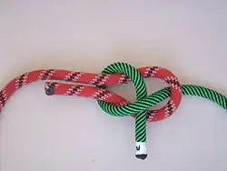
    The Eskimo bowline, Cossack knot (Russian: Казачий узел), reverse bowline, or ‘anti-bowline’ is in a class of knots known as ‘eye knots’ or ‘loop knots’. The eye is formed in the end of the rope to permit attachments/connections. It is quite common in Russia and is often used instead of the bowline (ABoK #1010). In the simple bowline, the collar component forms around the ‘standing part’. In contrast, the collar component of an Eskimo bowline forms around the outgoing eye-leg.

    On the first of arctic explorer John Ross’ expeditions (1818) the Inuit (Eskimos) presented him a sled that contained several of these knots, showing that it is a genuine Inuit knot.[1]
    The knot is not mentioned in The Ashley Book of Knots but in its Russian equivalent, the book “Морские узлы”
    [2]
    (Marine Knots) by Lev Skryagin (1930–2000). The knot is referred to in the Russian book as the Cossack knot, and its slipped version is known as the Kalmyk loop.

    Eskimo bowline
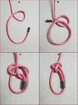
    Tying an Eskimo Bowline
    Eskimo bowline
    Eskimo bowline based on the method described by Geoffrey Budworth in The Illustrated Encyclopedia of Knots.[3] The tightened knot on the right takes on a trefoil crown shape.

    The Eskimo bowline is about as strong as and even more secure than the bowline,[4][1] especially in synthetic lines.

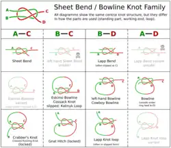
    Under cross load (ring loading, transverse loading profile), i.e. when the loop is pulled apart, the shown common Eskimo loop effectively mimics an ends-opposite (and inferior) left-hand sheet bend and thus can slip like the bowline; the less common Eskimo loop variant with the A–C loop (see bowline family diagram) would give a proper same-side sheet bend, thus being much stronger under cross load. Similarly, when the eye of a simple bowline is subject to a transverse loading profile, it mimics the inferior version of the Lapp bend, and so can slip and untie; the wrongly demeaned left-handed or cowboy bowline becomes the proper Lapp bend, and should hold..

    All of the maneuvers to tie this knot are generally in the opposite (or ‘anti’ direction) relative to the bowline. After forming the ‘nipping loop’ with C & D (which can be formed as ‘S’ or ‘Z’ chirality) the working end is fed through that loop from the same side A as the outgoing eye leg C. This is opposite (or ‘anti’) direction relative to the simple (ABOK #1010) Bowline (A–D on opposite sides).

    Eskimo bowline
    Sheet bend
    Eskimo bowline
    Bends and loops directly related to the sheet bend and bowline

    The so called ‘Eskimo’ Bowline has also been known as Boas Bowline and Cossack knot – all of these names referring to the same structure. The Kalmyk loop[5][6] can be made ‘TIB’ (Tiable In the Bight); however, it will not be ‘EEL’ (Either End Loadable).

    See also

    References

    1. 1 2 Budworth, Geoffrey (2001). The Complete Guide to Knot and Knot Tying. Lorenz Books. p. 179. ISBN 0-7548-0422-4.
    2. Skryagin, Lev (1994). Морские узлы. Транспорт. ISBN 5-277-01807-7.
    3. Budworth, Geoffrey (2002). The Illustrated Encyclopedia of Knots. Lyons Press. ISBN 978-1585746262.
    4. Compton, Nic (2013). The Knot Bible. Adlard Coles Nautical. p. 83. ISBN 978-1-4081-5476-2.
    5. Video on YouTube Tying video for Kalmyk loop
    6. Video on YouTube Tying video for Kalmyk loop

    External links


    This article is adapted from “Eskimo bowline” on Wikipedia, written by its contributors, and used under CC BY-SA 4.0. Text on this page is available under the same licence. Source snapshot: Wikipedia via Kiwix, 2026-07-20.

  • Three-twist knot

    Three-twist knot
    Three-twist knot
    Common name Figure-of-nine knot
    Arf invariant 0
    Braid length 6
    Braid no. 3
    Bridge no. 2
    Crosscap no. 2
    Crossing no. 5
    Genus 1
    Hyperbolic volume 2.82812
    Stick no. 8
    Unknotting no. 1
    Conway notation [32]
    A–B notation 52
    Dowker notation 4, 8, 10, 2, 6
    Last / Next 51 / 61
    Other
    alternating, hyperbolic, prime, reversible, twist

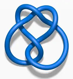
    In knot theory, the three-twist knot is the twist knot with three-half twists. It is listed as the 52 knot[1] in the Alexander-Briggs notation, and is one of two knots with crossing number five, the other being the cinquefoil knot.

    Properties

    The three-twist knot is a prime knot, and it is invertible but not amphichiral. Its Alexander polynomial is

    Δ ( t ) = 2 t 3 + 2 t 1 , {\displaystyle \Delta (t)=2t-3+2t^{-1},\,} {\displaystyle \Delta (t)=2t-3+2t^{-1},\,}

    since ( 1 1 0 2 ) {\displaystyle {\begin{pmatrix}1&-1\\0&2\end{pmatrix}}} {\displaystyle {\begin{pmatrix}1&-1\\0&2\end{pmatrix}}} is a possible Seifert matrix, or because of its Conway polynomial, which is

    ( z ) = 2 z 2 + 1 , {\displaystyle \nabla (z)=2z^{2}+1,\,} {\displaystyle \nabla (z)=2z^{2}+1,\,}

    and its Jones polynomial is

    V ( q ) = q 1 q 2 + 2 q 3 q 4 + q 5 q 6 . {\displaystyle V(q)=q^{-1}-q^{-2}+2q^{-3}-q^{-4}+q^{-5}-q^{-6}.\,} {\displaystyle V(q)=q^{-1}-q^{-2}+2q^{-3}-q^{-4}+q^{-5}-q^{-6}.\,}[2]

    Because the Alexander polynomial is not monic, the three-twist knot is not fibered.

    The three-twist knot is a hyperbolic knot, with its complement having a volume of approximately 2.82812.

    If the fibre of the knot in the initial image of this page were cut at the bottom right of the image, and the ends were pulled apart, it would result in a single-stranded figure-of-nine knot (not the figure-of-nine loop).

    Example

    References

    1. Pinsky, Tali (1 September 2017). “On the topology of the Lorenz system”. Proceedings of the Royal Society A: Mathematical, Physical and Engineering Sciences. 473 (2205) 20170374. The Royal Society. doi:10.1098/rspa.2017.0374. PMC 5627380. PMID 28989313. Retrieved 26 August 2018. (b) the knot with three half-twists, called the 52 knot.
    2. 5_2“, The Knot Atlas.

    This article is adapted from “Three-twist knot” on Wikipedia, written by its contributors, and used under CC BY-SA 4.0. Text on this page is available under the same licence. Source snapshot: Wikipedia via Kiwix, 2026-07-20.

  • Thief knot

    Thief knot
    Thief knot
    Names Thief knot, Bag knot, Bread bag knot
    Category Binding
    Origin Ancient
    Related Reef knot, Granny knot, Grief knot
    Releasing Jamming, but not always
    Caveat spills
    ABoK #1207

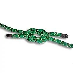
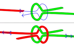
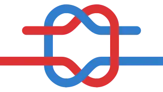
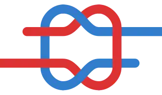
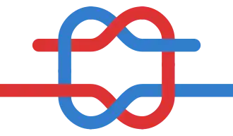
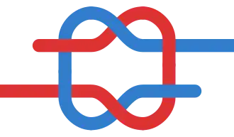
    The thief knot resembles the reef knot (square knot) except that the free, or bitter ends are on opposite sides. It is said that sailors would secure their belongings in a ditty bag using the thief knot, often with the ends hidden. If another sailor went through the bag, the odds were high the thief would tie the bag back using the more common reef knot, revealing the tampering, hence the name. It is difficult to tie by mistake, unlike the granny knot, unless one attempts to tie a square knot in a similar manner to a sheet bend (which is the correct way to tie a thief knot), then it is possible to tie accidentally.

    The thief knot is much less secure than the already insecure reef knot. It unties itself if the lines are pulled when the same action would seize a reef knot.[1]

    The thief or bag knot is also called bread bag knot. It appears very like the reef knot, but there is one real and scarcely evident difference. It does not consist of two half knots. There is a legend that sailors tie clothesbags, and bread bags with this knot and that thieves always retie them with reef knots and so are inevitably detected. It is a pleasing story that should encourage honesty. However, if I have ever met this knot in practical use, I have neither recognized it nor paid penalty for my failure to do so.

    Tying

    Thief knot
    Tying the thief knot step-by-step

    Related knots

    See also

    Sources

    1. Ashley, Clifford Warren (1950). The Ashley Book of Knots. Doubleday. p. 221. (knot number 1207)
    2. Ashley, Clifford W. (1944). The Ashley Book of Knots, p.221. Doubleday. ISBN 0-385-04025-3.

    External links


    This article is adapted from “Thief knot” on Wikipedia, written by its contributors, and used under CC BY-SA 4.0. Text on this page is available under the same licence. Source snapshot: Wikipedia via Kiwix, 2026-07-20.

  • Endless knot

    Endless knot
    Endless knot

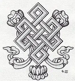
    A common form of the endless knot
    Chinese name
    Traditional Chinese 盤長結
    Simplified Chinese 盘长结
    Transcriptions
    Standard Mandarin
    Hanyu Pinyin pánzhǎng jié
    Tibetan name
    Tibetan དཔལ་བེའུ།
    Transcriptions
    Wylie dpal be’u
    Mongolian name
    Mongolian Cyrillic түмэн өлзий
    Japanese name
    Kanji 盤長結
    Transcriptions
    Romanization Banchōmusubi
    Sanskrit name
    Sanskrit श्रीवत्स
    Endless knot
    More decorative form of the endless knot
    Endless knot
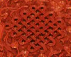
    More complex form of the endless knot is seen on a c. 400-year-old Chinese lacquerware dish
    Endless knot
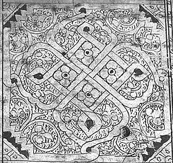
    Endless knot in a Burmese Pali manuscript

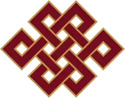
    In Hinduism, Jainism and Buddhism, the endless knot or eternal knot is a symbolic knot and one of the Eight Auspicious Symbols. It is an important cultural marker in places significantly influenced by Tibetan Buddhism such as Tibet, Mongolia, Tuva, Kalmykia, and Buryatia. It is also found in Celtic, Kazakh and Chinese symbolism.

    History

    The endless knot appears on clay tablets from the Indus Valley civilization (2500 BC)[1] and on a historic era inscription.[2] While associated with Dharmic religions, it also appears in Islamic art.[3][4] It likely was introduced due to trade and other cultural contact with China, the Mongols, and Iran.[5]

    Interpretations

    Buddhism

    Various Buddhist interpretations of the symbol are:

    • The endless knot iconography symbolised Samsara i.e., the endless cycle of suffering of birth, death and rebirth within Tibetan Buddhism.
    • The inter-twining of wisdom and compassion.
    • Interplay and interaction of the opposing forces in the dualistic world of manifestation, leading to their union, and ultimately to harmony in the universe.
    • The mutual dependence of religious doctrine and secular affairs.
    • The union of wisdom and method.
    • The inseparability of emptiness (shunyata) and dependent origination, the underlying reality of existence.
    • The link between ancestors and omnipresence represented by the etymology of Tantra, Yoga and religion) (see Namkha.)
    • The wisdom of the Buddha as neither are said to have a beginning or end.

    Hinduism

    In Hinduism, Srivatsa is mentioned as ‘connected to shree’, i.e the goddess Lakshmi. It is a mark on the chest of Vishnu where his consort Lakshmi resides. According to the Vishnu purana, the tenth avatar of Vishnu, Kalki, will bear the Shrivatsa mark on his chest. It is one of the names of Vishnu in the Vishnu Sahasranamam. Srivatsa is considered to be auspicious symbol in Andhra Pradesh, Telangana, Tamil Nadu and Karnataka.

    Jainism

    In Jainism it is one of the eight auspicious items, an asthamangala, however found only in the Svetambara sect. It is often found marking the chests of the 24 tirthankaras. It is more commonly referred to as the Shrivatsa.

    Logo

    A stylized version of the endless knot is the logo of the Chinese state-owned telecommunications operator China Unicom.

    See also

    Notes and references

    1. Beer, Robert (2003). The Handbook of Tibetan Buddhist Symbols (PDF). Serindia Publications. p. 11. ISBN 1-59030-100-5. Archived (PDF) from the original on 3 April 2018.
    2. Danino, Michel (2010). Lost River: On The Trail of the Sarasvati. Penguin Books. ISBN 978-0143068648.
    3. “Fragment of a Woodblock Print on Linen | Cleveland Museum of Art”. clevelandart.org. Retrieved 2024-07-22.
    4. “Pierced Globe”. The Metropolitan Museum of Art. Retrieved 2024-07-22.
    5. Blair, Sheila; Bloom, Jonathan; Ettinghausen, Richard (1994). The art and architecture of Islam 1250–1800. Yale University Press Pelican history of art. New Haven [Conn.]: Yale University Press. ISBN 978-0-300-05888-8.

    External links


      This article is adapted from “Endless knot” on Wikipedia, written by its contributors, and used under CC BY-SA 4.0. Text on this page is available under the same licence. Source snapshot: Wikipedia via Kiwix, 2026-07-20.

    • The Knot Atlas


      The Knot Atlas is a website, an encyclopedia rather than atlas, dedicated to knot theory. It and its predecessor were created by mathematician Dror Bar-Natan, who maintains the current site with Scott Morrison. According to Schiller, the site contains, “beautiful illustrations and detailed information about knots,” as does KnotPlot.com.[1] According to the site itself, it is a knot atlas (collection of maps), theory database, knowledge base, and “a home for some computer programs”.[2]

      References

      1. Schiller, Christoph (2012). Motion Mountain, The Adventure of Physics – Vol. 5: Motion Inside Matter – Pleasure, Technology and Stars, p. 272. MotionMountain.net.
      2. Official website Edit this at Wikidata

      External links


      This article is adapted from “The Knot Atlas” on Wikipedia, written by its contributors, and used under CC BY-SA 4.0. Text on this page is available under the same licence. Source snapshot: Wikipedia via Kiwix, 2026-07-20.

    • Eilenberg–Mazur swindle

      In mathematics, the Eilenberg–Mazur swindle, named after Samuel Eilenberg and Barry Mazur, is a method of proof that involves paradoxical properties of infinite sums. In geometric topology, it was introduced by Mazur[1][2] and is often called the Mazur swindle. In algebra, it was introduced by Samuel Eilenberg and is known as the Eilenberg swindle or Eilenberg telescope (see telescoping sum).

      The Eilenberg–Mazur swindle is similar to the following well known joke “proof” that 1 = 0:

      1 = 1 + (1 + 1) + (1 + 1) +  = 1  1 + 1  1 +  = (1  1) + (1  1) +  = 0

      This “proof” is not valid as a claim about real numbers because Grandi’s series 1  1 + 1  1 + … does not converge, but the analogous argument can be used in some contexts where there is some sort of “addition” defined on some objects for which infinite sums do make sense,
      to show that if A + B = 0 {\displaystyle A+B=0} {\displaystyle A+B=0} then A = B = 0 {\displaystyle A=B=0} {\displaystyle A=B=0}.

      Mazur swindle

      In geometric topology, the addition used in the swindle is usually the connected sum of knots or manifolds.

      A typical application of the Mazur swindle is the proof that the sum of two non-trivial knots A {\displaystyle A} {\displaystyle A} and B {\displaystyle B} {\displaystyle B} is non-trivial.[3] For knots it is possible to take infinite sums by making the knots smaller and smaller, so if A + B {\displaystyle A+B} {\displaystyle A+B} is trivial then

      A = A + ( B + A ) + ( B + A ) + = ( A + B ) + ( A + B ) + = 0 {\displaystyle A=A+(B+A)+(B+A)+\cdots =(A+B)+(A+B)+\cdots =0} {\displaystyle A=A+(B+A)+(B+A)+\cdots =(A+B)+(A+B)+\cdots =0}

      so A {\displaystyle A} {\displaystyle A} is trivial (and B {\displaystyle B} {\displaystyle B} by an analogous argument). The infinite sum of knots is usually a wild knot, not a tame knot. There are many geometric examples of the swindle.[4]

      Oriented n {\displaystyle n} {\displaystyle n}-manifolds have an addition operation given by connected sum, with identity the n {\displaystyle n} {\displaystyle n}-sphere. If A + B {\displaystyle A+B} {\displaystyle A+B} is the n {\displaystyle n} {\displaystyle n}-sphere, then A + B + A + B + {\displaystyle A+B+A+B+\cdots } {\displaystyle A+B+A+B+\cdots } is Euclidean space, so the Mazur swindle shows that the connected sum of A {\displaystyle A} {\displaystyle A} and Euclidean space is again Euclidean space. Hence A {\displaystyle A} {\displaystyle A} is the one-point compactification of Euclidean space and therefore A {\displaystyle A} {\displaystyle A} is homeomorphic to the n {\displaystyle n} {\displaystyle n}-sphere. (This does not show in the case of smooth manifolds that A {\displaystyle A} {\displaystyle A} is diffeomorphic to the n {\displaystyle n} {\displaystyle n}-sphere, and in some dimensions, such as 7 {\displaystyle 7} {\displaystyle 7}, there are examples of exotic spheres A {\displaystyle A} {\displaystyle A} with inverses that are not diffeomorphic to the standard n {\displaystyle n} {\displaystyle n}-sphere.)

      Eilenberg swindle

      In algebra the addition used in the swindle is usually the direct sum of modules over a ring.

      A typical application of the Eilenberg swindle in algebra is the proof that if A {\displaystyle A} {\displaystyle A} is a projective module over a ring R {\displaystyle R} {\displaystyle R} then there is a free module F {\displaystyle F} {\displaystyle F} with A F F {\displaystyle A\oplus F\cong F} {\displaystyle A\oplus F\cong F}.[5][6] To see this, choose a module B {\displaystyle B} {\displaystyle B} such that A B {\displaystyle A\oplus B} {\displaystyle A\oplus B} is free, which can be done as A {\displaystyle A} {\displaystyle A} is projective, and put

      F = B A B A B {\displaystyle F=B\oplus A\oplus B\oplus A\oplus B\oplus \cdots } {\displaystyle F=B\oplus A\oplus B\oplus A\oplus B\oplus \cdots }

      so that

      A F = A ( B A ) ( B A ) = ( A B ) ( A B ) F . {\displaystyle A\oplus F=A\oplus (B\oplus A)\oplus (B\oplus A)\oplus \cdots =(A\oplus B)\oplus (A\oplus B)\oplus \cdots \cong F.} {\displaystyle A\oplus F=A\oplus (B\oplus A)\oplus (B\oplus A)\oplus \cdots =(A\oplus B)\oplus (A\oplus B)\oplus \cdots \cong F.}

      For another application of the swindle, recall that finitely-generated free modules over commutative rings have a well-defined natural number as their dimension which is additive under direct sums, and are isomorphic if and only if they have the same dimension.[7]

      This is false for some noncommutative rings, and a counterexample can be constructed using the Eilenberg swindle as follows: let X {\displaystyle X} {\displaystyle X} be an abelian group such that X X X {\displaystyle X\cong X\oplus X} {\displaystyle X\cong X\oplus X} (for example the direct sum of an infinite number of copies of any nonzero abelian group), and let R {\displaystyle R} {\displaystyle R} be the ring of endomorphisms of X {\displaystyle X} {\displaystyle X}. Then the left R {\displaystyle R} {\displaystyle R}-module R {\displaystyle R} {\displaystyle R} is isomorphic to the left R {\displaystyle R} {\displaystyle R}-module R R {\displaystyle R\oplus R} {\displaystyle R\oplus R}.

      As a final interesting example,[8] if A {\displaystyle A} {\displaystyle A} and B {\displaystyle B} {\displaystyle B} are any groups then the Eilenberg swindle can be used to construct a ring R {\displaystyle R} {\displaystyle R} such that the group rings R [ A ] {\displaystyle R[A]} {\displaystyle R[A]} and R [ B ] {\displaystyle R[B]} {\displaystyle R[B]} are isomorphic rings: take R {\displaystyle R} {\displaystyle R} to be the group ring of the restricted direct product of infinitely many copies of A × B {\displaystyle A\times B} {\displaystyle A\times B}.

      Other examples

      The proof of the Schröder-Bernstein theorem might be seen as antecedent of the Eilenberg–Mazur swindle. In fact, the ideas are quite similar. If there are injections of sets from X to Y and from Y to X, this means that formally we have X = Y + A and Y = X + B for some sets A and B, where + means disjoint union and = means there is a bijection between two sets. Expanding the former with the latter,

      X = X + A + B.

      In this bijection, let Z consist of those elements of the left hand side that correspond to an element of X on the right hand side. This bijection then expands to the bijection

      X = A + B + A + B + ⋯ + Z.

      Substituting the right hand side for X in Y = B + X gives the bijection

      Y = B + A + B + A + ⋯ + Z.

      Switching every adjacent pair B + A yields

      Y = A + B + A + B + ⋯ + Z.

      Composing the bijection for X with the inverse of the bijection for Y then yields

      X = Y.

      This argument depended on the bijections A + B = B + A and A + (B + C) = (A + B) + C as well as the well-definedness of infinite disjoint union.

      Notes

      1. Mazur (1959).
      2. Mazur (1961).
      3. Rolfsen (1976), chapter 4B.
      4. Poénaru (2007).
      5. Lam (1999), p. 22, corollary 2.7.
      6. Eklof & Mekler (2002), p. 9, lemma 2.3.
      7. Eisenbud (1995), p. 121.
      8. Lam (2003), exercise 8.16.

      References

      • Eisenbud, David (1995). Commutative Algebra. Graduate Texts in Mathematics. Vol. 150. New York: Springer. ISBN 978-0-387-94268-1. MR 1322960.
      • Eklof, Paul C.; Mekler, Alan H. (2002) [1990]. Almost Free Modules: Set-Theoretic Models. North Holland Mathematical Library. Vol. 65 (revised ed.). Amsterdam: Elsevier. ISBN 0-444-88502-1.
      • Lam, Tsit-Yuen (2003). Exercises in Classical Ring Theory. Problem Books in Mathematics. New York: Springer. ISBN 978-0-387-00500-3.
      • Lam, Tsit-Yuen (1999). Lectures on Modules and Rings. Graduate Texts in Mathematics. Vol. 189. New York: Springer. ISBN 978-0-387-98428-5.
      • Mazur, Barry (1959). “On the structure of certain semi-groups of spherical knot classes”. Publications Mathématiques de l’IHÉS. 3: 19–27. doi:10.1007/bf02684388. MR 0116347.
      • Mazur, B. C. (1961). “On embeddings of spheres”. Acta Mathematica. 105 (1–2): 1–17. doi:10.1007/BF02559532. MR 0125570.
      • Rolfsen, Dale (1976). Knots and Links. Berkeley: Publish or Perish. ISBN 0-914098-16-0.

      External links


      This article is adapted from “Eilenberg–Mazur swindle” on Wikipedia, written by its contributors, and used under CC BY-SA 4.0. Text on this page is available under the same licence. Source snapshot: Wikipedia via Kiwix, 2026-07-20.

    • The Ashley Book of Knots

      The Ashley Book of Knots
      The Ashley Book of Knots

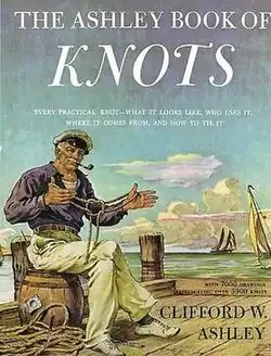
      Cover illustration by George Giguere shows a sailor displaying a Tom fool’s knot
      Author Clifford W. Ashley
      Illustrator Clifford W. Ashley
      Cover artist George Giguere
      Language English
      Subject Knots
      Genre Reference work
      Publisher Doubleday
      Publication date 1944
      Publication place United States
      Pages 638
      ISBN 0-385-04025-3
      The Ashley Book of Knots
      Reprint-Version: 1963–1979

      The Ashley Book of Knots (ABoK) is an encyclopedia of knots written and illustrated by the American sailor and artist Clifford W. Ashley. First published in 1944, it was the culmination of over 11 years of work. The book contains 3,857 numbered entries and approximately 7,000 illustrations.[1] The entries include knot instructions, uses, and some histories, categorized by type or function. It remains one of the most important and comprehensive books on knots.

      Use as a reference

      Due to its scope and wide availability, The Ashley Book of Knots has become a significant reference work in the field of knotting. The numbers Ashley assigned to each knot can be used to unambiguously identify them. This helps to identify knots despite local colloquialisms or identification changes. Citations to Ashley numbers are usually in the form: “The Constrictor Knot (ABoK #1249)”, “ABoK #1249”, or even simply “#1249” if the context of the reference is clear or already established.[2]

      Some knots have more than one Ashley number due to having multiple uses or forms. For example, the main entry for #1249 is in the chapter on binding knots but it is also listed as #176 in a chapter on occupational knot usage.

      The Ashley Book of Knots was compiled and first published before the introduction of synthetic fiber ropes, during a time when natural fiber cordage – typically twisted, laid, or braided rope – was most commonly used. The commentary on some knots may fail to address their behavior when tied with modern synthetic fiber or kernmantle style ropes.

      Corrections and additions

      In the first edition, three entries have non-integer numbers: 794.5,  1034.5,  2585.5. 
      Also, entry number 2545 contains no knot, reading only “This knot was mislaid”.[1]

      Ashley suffered a debilitating stroke the year after the book was published.[3] He was not able to produce an erratum nor oversee a corrected edition.

      In 1979, at least one knot was added, the Hunter’s bend (#1425A).[4]

      In 1991, corrections submitted by the International Guild of Knot Tyers were incorporated.[5][6] The original list of revisions submitted to the publisher is believed to have been lost, but many had been collected from a series of articles in Knotting Matters, the Guild’s quarterly publication.[7][8] Additional errors have been identified since the 1991 corrections.[9]

      Cultural references

      The Ashley Book of Knots is quoted extensively in the novel The Shipping News (1993) by E. Annie Proulx, with its descriptions and illustrations of various knots providing the chapter headings. In the novel’s acknowledgements, Proulx writes that “without the inspiration of Clifford W. Ashley’s wonderful 1944 work, The Ashley Book of Knots, which I had the good fortune to find at a yard sale for a quarter, this book would have remained just a thread of an idea.”

      Notes and references

      1. 1 2 Ashley, Clifford W. (1993) [1944], The Ashley Book of Knots, New York: Doubleday, p. Dust jacket, ISBN 0-385-04025-3
      2. Warner, Charles; Turner, John (1996), Turner, J.C.; van de Griend, P. (eds.), History and Science of Knots, K&E Series on Knots and Everything, vol. 11, Singapore: World Scientific Publishing, pp. 22, 274–275, ISBN 981-02-2469-9
      3. Budworth, Geoffrey, ed. (Spring 1985). “Profile of Knotsman Clifford W. Ashley”. Knotting Matters (11). London: International Guild of Knot Tyers: 6–7. ISSN 0959-2881.
      4. Ashley (1993), pp. 260–261
      5. Budworth, Geoffrey (Autumn 1991). “Amending Ashley”. Knotting Matters (37). London: International Guild of Knot Tyers: 26. ISSN 0959-2881.
      6. Ashley (1993), p. Edition notice
      7. Schmidbauer, Joseph, ed. (September 1998), “The Ashley Book of Knots: Corrections and Observations”, Knot News (13), International Guild of Knot Tyers – Pacific Americas Branch: 1–3
      8. The Knotting Matters issues cited in the above Knot News article are: KM1, KM28, KM31, KM32, and KM33.
      9. For an example see the footnotes in harness loop and butterfly loop articles. Additionally, this IGKT posting contains many verifiable examples.

      Further reading

      • Clifford W. Ashley. The Ashley Book of Knots. Doubleday, New York 1944. ISBN 0-385-04025-3
      • Reprint: Doubleday, New York 1963–1979, ISBN 0-571-09659-X
      • Reprint with amendment of Geoffrey Budworth: The Ashley Book of Knots. With amendments of Geoffrey Budworth. Doubleday, New York 1993.

      External links


      This article is adapted from “The Ashley Book of Knots” on Wikipedia, written by its contributors, and used under CC BY-SA 4.0. Text on this page is available under the same licence. Source snapshot: Wikipedia via Kiwix, 2026-07-20.