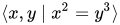
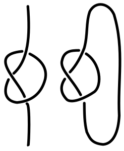
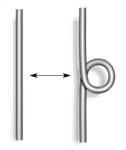
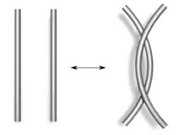
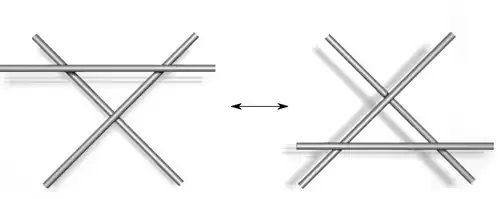
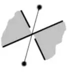
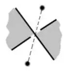
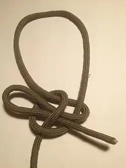
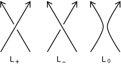
Many knot polynomials are computed using skein relations, which allow one to change the different crossings of a knot to get simpler knots.
In the mathematical field of knot theory, a knot polynomial is a knot invariant in the form of a polynomial whose coefficients encode some of the properties of a given knot.
History
The first knot polynomial, the Alexander polynomial, was introduced by James Waddell Alexander II in 1923. Other knot polynomials were not found until almost 60 years later.
In the 1960s, John Conway came up with a skein relation for a version of the Alexander polynomial, usually referred to as the Alexander–Conway polynomial. The significance of this skein relation was not realized until the early 1980s, when Vaughan Jones discovered the Jones polynomial. This led to the discovery of more knot polynomials, such as the so-called HOMFLY polynomial.
Soon after Jones’ discovery, Louis Kauffman noticed the Jones polynomial could be computed by means of a partition function (state-sum model), which involved the bracket polynomial, an invariant of framed knots. This opened up avenues of research linking knot theory and statistical mechanics.
In the late 1980s, two related breakthroughs were made. Edward Witten demonstrated that the Jones polynomial, and similar Jones-type invariants, had an interpretation in Chern–Simons theory. Viktor Vasilyev and Mikhail Goussarov started the theory of finite type invariants of knots. The coefficients of the previously named polynomials are known to be of finite type (after perhaps a suitable “change of variables”).
In recent years, the Alexander polynomial has been shown to be related to Floer homology. The graded Euler characteristic of the knot Floer homology of Peter Ozsváth and Zoltan Szabó is the Alexander polynomial.
Graph polynomial, a similar class of polynomial invariants in graph theory
Tutte polynomial, a special type of graph polynomial related to the Jones polynomial
Skein relation for a formal definition of the Alexander polynomial, with a worked-out example.
Further reading
Adams, Colin. The Knot Book. American Mathematical Society. ISBN0-8050-7380-9.
Lickorish, W. B. R. (1997). An Introduction to Knot Theory. Graduate Texts in Mathematics. Vol.175. New York: Springer-Verlag. ISBN0-387-98254-X.
This article is adapted from “Knot polynomial” on Wikipedia, written by its contributors, and used under CC BY-SA 4.0. Text on this page is available under the same licence. Source snapshot: Wikipedia via Kiwix, 2026-07-20.
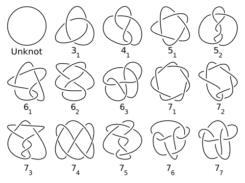
Prime knots are organized by the crossing number invariant.
In the mathematical field of knot theory, a knot invariant is a quantity (in a broad sense) defined for each knot which is the same for equivalent knots. The equivalence is often given by ambient isotopy but can be given by homeomorphism.[1] Some invariants are indeed numbers (algebraic[2]), but invariants can range from the simple, such as a yes/no answer, to those as complex as a homology theory (for example, “a knot invariant is a rule that assigns to any knot K a quantity φ(K) such that if K and K’ are equivalent then φ(K) = φ(K’).”[3]). Research on invariants is not only motivated by the basic problem of distinguishing one knot from another but also to understand fundamental properties of knots and their relations to other branches of mathematics. Knot invariants are thus used in knot classification,[3][4] both in “enumeration” and “duplication removal”.[2]
A knot invariant is a quantity defined on the set of all knots, which takes the same value for any two equivalent knots. For example, a knot group is a knot invariant.[5]
General properties
Typically a knot invariant is a combinatorial quantity defined on knot diagrams. Thus if two knot diagrams differ with respect to some knot invariant, they must represent different knots. However, as is generally the case with topological invariants, if two knot diagrams share the same values with respect to a [single] knot invariant, then we still cannot conclude that the knots are the same.[6]
Invariants from knot diagrams
From the modern perspective, it is natural to define a knot invariant from a knot diagram. Of course, it must be unchanged (that is to say, invariant) under the Reidemeister moves (“triangular moves”[4]). Tricolorability (and n-colorability) is a particularly simple and common example. Other examples are knot polynomials, such as the Jones polynomial, which are currently among the most useful invariants for distinguishing knots from one another, though currently it is not known whether there exists a knot polynomial which distinguishes all knots from each other.[7][8][9] However, there are invariants which distinguish the unknot from all other knots, such as Khovanov homology and knot Floer homology.
Extremal diagram invariants
Other invariants can be defined by considering some integer-valued function of knot diagrams and taking its minimum value over all possible diagrams of a given knot. This category includes the crossing number, which is the minimum number of crossings for any diagram of the knot, and the bridge number, which is the minimum number of bridges for any diagram of the knot.
Classical and intrinsic invariants
Historically, many of the early knot invariants are not defined by first selecting a diagram but defined intrinsically, which can make computing some of these invariants a challenge. For example, knot genus is particularly tricky to compute, but can be effective (for instance, in distinguishing mutants).
Complete invariants
The complement of a knot itself (as a topological space) is known to be a “complete invariant” of the knot by the Gordon–Luecke theorem in the sense that it distinguishes the given knot from all other knots up to ambient isotopy and mirror image. Some invariants associated with the knot complement include the knot group which is just the fundamental group of the complement. The knot quandle is also a complete invariant in this sense but it is difficult to determine if two quandles are isomorphic. The peripheral subgroup can also work as a complete invariant.[10]
Hyperbolic invariants
By Mostow–Prasad rigidity, the hyperbolic structure on the complement of a hyperbolic link is unique, which means the hyperbolic volume is an invariant for these knots and links. Volume, and other hyperbolic invariants, have proven very effective, utilized in some of the extensive efforts at knot tabulation.
Homological invariants
In recent years, there has been much interest in homological invariants of knots which categorify well-known invariants. Heegaard Floer homology is a homology theory whose Euler characteristic is the Alexander polynomial of the knot. It has been proven effective in deducing new results about the classical invariants. Along a different line of study, there is a combinatorially defined cohomology theory of knots called Khovanov homology whose Euler characteristic is the Jones polynomial. This has recently been shown to be useful in obtaining bounds on slice genus whose earlier proofs required gauge theory. Mikhail Khovanov and Lev Rozansky have since defined several other related cohomology theories whose Euler characteristics recover other classical invariants. Catharina Stroppel gave a representation theoretic interpretation of Khovanov homology by categorifying quantum group invariants.
Physical and geometric invariants
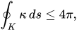
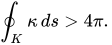
There is also growing interest from both knot theorists and scientists in understanding “physical” or geometric properties of knots and relating it to topological invariants and knot type. An old result in this direction is the Fáry–Milnor theorem states that if the total curvature of a knot K in satisfies
where κ(p) is the curvature at p, then K is an unknot. Therefore, for knotted curves,
An example of a “physical” invariant is ropelength, which is the length of unit-diameter rope needed to realize a particular knot type.
Other invariants
Linking number– How many times curves wind around each other
Finite type invariant– Type of invariant in Knot theory (or Vassiliev or Vassiliev–Goussarov invariant)
Stick number– Smallest number of edges of an equivalent polygonal path for a knot
Arnold invariants– Mathematical invariants used to classify plane curves
Sources
↑Schultens, Jennifer (2014). Introduction to 3-manifolds, p.113. American Mathematical Society. ISBN9781470410209
12Ricca, Renzo L.; ed. (2012). An Introduction to the Geometry and Topology of Fluid Flows, p.67. Springer Netherlands. ISBN9789401004466.
12Purcell, Jessica (2020). Hyperbolic Knot Theory, p.7. American Mathematical Society. ISBN9781470454999 “A knot invariant is a function from the set of knots to some other set whose value depends only on the equivalence class of the knot.”
12Messer, Robert and Straffin, Philip D. (2018). Topology Now!, p.50. American Mathematical Society. ISBN9781470447816 “A knot invariant is a mathematical property or quantity associated with a knot that does not change as we perform triangular moves on the knot.
↑Morishita, Masanori (2011). Knots and Primes: An Introduction to Arithmetic Topology, p.16. Springer London. ISBN9781447121589. “Likewise,” with knot invariants, “a quantity inv(L) = inv(L’) for any two equivalent links L and L’.”
↑Ault, Shaun V. (2018). Understanding Topology: A Practical Introduction, p.245. Johns Hopkins University Press. ISBN9781421424071.
↑Skerritt, Matt (June 27, 2003). “An Introduction to Knot Theory”(PDF). carmamaths.org. p.22. Archived(PDF) from the original on November 19, 2022. Retrieved November 19, 2022.
↑Hodorog, Mădălina (February 2, 2010). “Basic Knot Theory”(PDF). www.dk-compmath.jku.at/people/mhodorog/. p.47. Archived(PDF) from the original on November 19, 2022. Retrieved November 19, 2022.
Rolfsen, Dale (2003). Knots and Links. Providence, RI: AMS. ISBN0-8218-3436-3.
Adams, Colin Conrad (2004). The Knot Book: an Elementary Introduction to the Mathematical Theory of Knots (Repr., with corred.). Providence, RI: AMS. ISBN0-8218-3678-1.
Burde, Gerhard; Zieschang, Heiner (2002). Knots (2nd rev. and extendeded.). New York: De Gruyter. ISBN3-11-017005-1.
This article is adapted from “Knot invariant” on Wikipedia, written by its contributors, and used under CC BY-SA 4.0. Text on this page is available under the same licence. Source snapshot: Wikipedia via Kiwix, 2026-07-20.
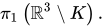
In mathematics, a knot is an embedding of a circle into 3-dimensional Euclidean space. The knot group of a knot K is defined as the fundamental group of the knot complement of K in R3,
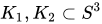
Other conventions consider knots to be embedded in the 3-sphere, in which case the knot group is the fundamental group of its complement in .
Properties
Two equivalent knots have isomorphic knot groups, so the knot group is a knot invariant and can be used to distinguish between certain pairs of inequivalent knots. This is because an equivalence between two knots is a self-homeomorphism of that is isotopic to the identity and sends the first knot onto the second. Such a homeomorphism restricts onto a homeomorphism of the complements of the knots, and this restricted homeomorphism induces an isomorphism of fundamental groups. However, it is possible for two inequivalent knots to have isomorphic knot groups (see below for an example).
The abelianization of a knot group is always isomorphic to the infinite cyclic group Z; this follows because the abelianization agrees with the first homology group, which can be easily computed.
The knot group (or fundamental group of an oriented link in general) can be computed in the Wirtinger presentation by a relatively simple algorithm.
Hazewinkel, Michiel, ed. (2001), “Knot and Link Groups“, Encyclopedia of Mathematics, Springer, ISBN978-1556080104
This article is adapted from “Knot group” on Wikipedia, written by its contributors, and used under CC BY-SA 4.0. Text on this page is available under the same licence. Source snapshot: Wikipedia via Kiwix, 2026-07-20.
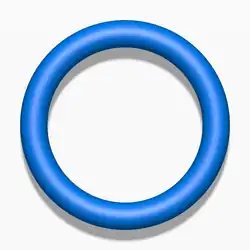
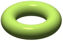
The knot complement of the unknot is homeomorphic to a solid torus – notice that while the unknot itself can be represented as a torus, the hole in the unknot corresponds to the solid region of the complement, while the knot itself is the hole in the complement. This is connected to the trivial Heegaard decomposition of the 3-sphere into two solid tori.
In mathematics, the knot complement of a tame knotK is the space where the knot is not. If a knot is embedded in the 3-sphere, then the complement is the 3-sphere minus the space near the knot. To make this precise, suppose that K is a knot in a three-manifold M (most often, M is the 3-sphere). Let N be a tubular neighborhood of K; so N is a solid torus. The knot complement is then the complement of N,
The knot complement XK is a compact 3-manifold; the boundary of XK and the boundary of the neighborhood N are homeomorphic to a two-torus. Sometimes the ambient manifold M is understood to be the 3-sphere. Context is needed to determine the usage. There are analogous definitions for the link complement.
Many knot invariants, such as the knot group, are really invariants of the complement of the knot. When the ambient space is the three-sphere no information is lost: the Gordon–Luecke theorem states that a knot is determined by its complement. That is, if K and K′ are two knots with homeomorphic complements then there is a homeomorphism of the three-sphere taking one knot to the other.
Knot complements are Haken manifolds.[1] More generally complements of links are Haken manifolds.
This article is adapted from “Knot complement” on Wikipedia, written by its contributors, and used under CC BY-SA 4.0. Text on this page is available under the same licence. Source snapshot: Wikipedia via Kiwix, 2026-07-20.
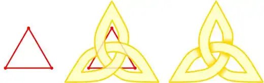
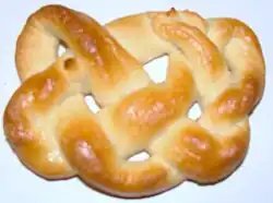
A table of all prime knots with seven crossings or fewer (not including mirror images)An overhand knot becomes a trefoil knot by joining the ends.The triangle is associated with the trefoil knot.Pretzel bread in the shape of a 74pretzel knot
In mathematics, a knot is an embedding of the circle (S1) into three-dimensional Euclidean space, R3 (also known as E3). Often two knots are considered equivalent if they are ambient isotopic, that is, if there exists a continuous deformation of R3 which takes one knot to the other.
A crucial difference between the standard mathematical and conventional notions of a knot is that mathematical knots are closed — there are no ends to tie or untie on a mathematical knot. Physical properties such as friction and thickness also do not apply, although there are mathematical definitions of a knot that take such properties into account. The term knot is also applied to embeddings of Sj in Sn, especially in the case j = n − 2. The branch of mathematics that studies knots is known as knot theory and has many relations to graph theory.
Formal definition
A knot is an embedding of the circle (S1) into three-dimensional Euclidean space (R3),[1] or the 3-sphere (S3), since the 3-sphere is compact.[2][Note 1] Two knots are defined to be equivalent if there is an ambient isotopy between them.[3]
Projection
A knot in R3 (or alternatively in the 3-sphere,S3), can be projected onto a planeR2 (respectively a sphereS2). This projection is almost always regular, meaning that it is injective everywhere, except at a finite number of crossing points, which are the projections of only two points of the knot, and these points are not collinear. In this case, by choosing a projection side, one can completely encode the isotopy class of the knot by its regular projection by recording a simple over/under information at these crossings. In graph theory terms, a regular projection of a knot, or knot diagram is thus a quadrivalent planar graph with over/under-decorated vertices. The local modifications of this graph which allow to go from one diagram to any other diagram of the same knot (up to ambient isotopy of the plane) are called Reidemeister moves.
Reidemeister move 1
Reidemeister move 2
Reidemeister move 3
Types of knots
A knot can be untied if the loop is broken.
The simplest knot, called the unknot or trivial knot, is a round circle embedded in R3.[4] In the ordinary sense of the word, the unknot is not “knotted” at all. The simplest nontrivial knots are the trefoil knot (31 in the table), the figure-eight knot (41) and the cinquefoil knot (51).[5]
Several knots, linked or tangled together, are called links. Knots are links with a single component.
Tame vs. wild knots
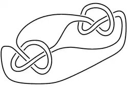
A wild knot
A polygonal knot is a knot whose image in R3 is the union of a finite set of line segments.[6] A tame knot is any knot equivalent to a polygonal knot.[6][Note 2] Knots which are not tame are called wild,[7] and can have pathological behavior.[7] In knot theory and 3-manifold theory, often the adjective “tame” is omitted. Smooth knots, for example, are always tame.
Framed knot
A framed knot is the extension of a tame knot to an embedding of the solid torus D2 × S1 in S3.
The framing of the knot is the linking number of the image of the ribbon I × S1 with the knot. A framed knot can be seen as the embedded ribbon and the framing is the (signed) number of twists.[8] This definition generalizes to an analogous one for framed links. Framed links are said to be equivalent if their extensions to solid tori are ambient isotopic.
Framed link diagrams are link diagrams with each component marked, to indicate framing, by an integer representing a slope with respect to the meridian and preferred longitude. A standard way to view a link diagram without markings as representing a framed link is to use the blackboard framing. This framing is obtained by converting each component to a ribbon lying flat on the plane. A type I Reidemeister move clearly changes the blackboard framing (it changes the number of twists in a ribbon), but the other two moves do not. Replacing the type I move by a modified type I move gives a result for link diagrams with blackboard framing similar to the Reidemeister theorem: Link diagrams, with blackboard framing, represent equivalent framed links if and only if they are connected by a sequence of (modified) type I, II, and III moves.
Given a knot, one can define infinitely many framings on it.
Suppose that we are given a knot with a fixed framing.
One may obtain a new framing from the existing one by cutting a ribbon and twisting it an integer multiple of 2π around the knot and then glue back again in the place we did the cut.
In this way one obtains a new framing from an old one, up to the equivalence relation for framed knots, leaving the knot fixed.[9] The framing in this sense is associated to the number of twists
the vector field performs around the knot. Knowing how many times the vector field is twisted around
the knot allows one to determine the vector field up to diffeomorphism, and the equivalence class of the
framing is determined completely by this integer called the framing integer.
Knot complement
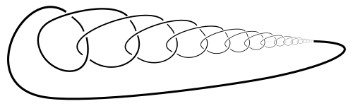
A knot whose complement has a non-trivial JSJ decomposition
Given a knot in the 3-sphere, the knot complement is all the points of the 3-sphere not contained in the knot. A major theorem of Gordon and Luecke states that at most two knots have homeomorphic complements (the original knot and its mirror reflection). This in effect turns the study of knots into the study of their complements, and in turn into 3-manifold theory.[10]
JSJ decomposition
The JSJ decomposition and Thurston’s hyperbolization theorem reduces the study of knots in the 3-sphere to the study of various geometric manifolds via splicing or satellite operations. In the pictured knot, the JSJ-decomposition splits the complement into the union of three manifolds: two trefoil complements and the complement of the Borromean rings. The trefoil complement has the geometry of H2 × R, while the Borromean rings complement has the geometry of H3.
Harmonic knots
Parametric representations of knots are called harmonic knots. Aaron Trautwein compiled parametric representations for all knots up to and including those with a crossing number of 8 in his PhD thesis.[11][12]
Connected Sum
In knot theory, the connected sum (or knot sum) of two oriented knots is the natural way to combine them. It makes the set of oriented knot types into a commutative monoid with the unknot as identity, and the operation is central to the decomposition of knots into prime pieces.
Definition
Let be two oriented, tame knots. Choose a 3‑ball that meets in a single unknotted arc. Remove the interior of a smaller arc‑neighbourhood from each ball, obtaining a pair whose boundary sphere intersects the knot in two points. The connected sum is formed by gluing the exteriors and along their boundary spheres via an orientation‑reversing homeomorphism that matches the endpoints of the arcs and preserves the given orientations. The result is again , and the image of the two arcs is a new oriented knot.
The construction does not depend on the choices of balls, arcs, or gluing map; any two connected sums of the same oriented knots are isotopic. In practice one often draws the connected sum by taking knot diagrams of the two knots, cutting a small arc from each diagram and joining the loose ends without introducing new crossings, respecting orientations.
If the knots are not oriented, the result may depend on the relative orientation, because some knots are non‑invertible. Standard practice is to work with oriented knots.
Properties
Well‑definedness: is a unique knot type for oriented knots.
No inverses: If is non‑trivial, there is no knot such that . Hence oriented knot types form a monoid, not a group.
Genus: The knot genus is additive: . Thus a connected sum of non‑trivial knots is non‑trivial.
Crossing number: The crossing number is subadditive: . It is an open problem whether equality always holds.
Prime knots and Schubert’s theorem
A knot is prime if it is non‑trivial and not a connected sum of two non‑trivial knots. The fundamental theorem, proved by Horst Schubert in 1949, states:
Every non‑trivial oriented knot decomposes as a connected sum of prime knots. The decomposition is unique up to the order of the factors.
Thus the monoid of oriented knot types is a free commutative monoid on the set of prime knots. The unknot plays the role of the unit, analogous to the number 1. For links of more than one component, unique decomposition fails.
Behaviour of invariants
Many polynomial and homological invariants are multiplicative under the connected sum:
The multiplicativity of the Alexander, Jones, and HOMFLY polynomials follows immediately from the skein relations.
Connected sum of links
For ordered links, the connected sum can be performed on chosen components, but the result depends on the choice of components and the ordering. Unlike for knots, the monoid of links is not free and factorisation into prime links is not unique.
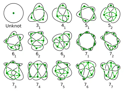
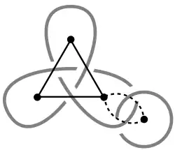
The signed planar graph associated with a knot diagram.Left guideRight guide
Another convenient representation of knot diagrams [13][14] was introduced by Peter Tait in 1877.[15][16]
Any knot diagram defines a plane graph whose vertices are the crossings and whose edges are paths in between successive crossings. Exactly one face of this planar graph is unbounded; each of the others is homeomorphic to a 2-dimensional disk. Color these faces black or white so that the unbounded face is black and any two faces that share a boundary edge have opposite colors. The Jordan curve theorem implies that there is exactly one such coloring.
We construct a new plane graph whose vertices are the white faces and whose edges correspond to crossings. We can label each edge in this graph as a left edge or a right edge, depending on which thread appears to go over the other as we view the corresponding crossing from one of the endpoints of the edge. Left and right edges are typically indicated by labeling left edges + and right edges –, or by drawing left edges with solid lines and right edges with dashed lines.
The original knot diagram is the medial graph of this new plane graph, with the type of each crossing determined by the sign of the corresponding edge. Changing the sign of every edge corresponds to reflecting the knot in a mirror.
Linkless and knotless embedding
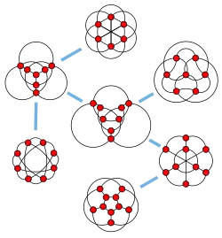
The seven graphs in the Petersen family. No matter how these graphs are embedded into three-dimensional space, some two cycles will have nonzero linking number.
In two dimensions, only the planar graphs may be embedded into the Euclidean plane without crossings, but in three dimensions, any undirected graph may be embedded into space without crossings. However, a spatial analogue of the planar graphs is provided by the graphs with linkless embeddings and knotless embeddings. A linkless embedding is an embedding of the graph with the property that any two cycles are unlinked; a knotless embedding is an embedding of the graph with the property that any single cycle is unknotted. The graphs that have linkless embeddings have a forbidden graph characterization involving the Petersen family, a set of seven graphs that are intrinsically linked: no matter how they are embedded, some two cycles will be linked with each other.[17] A full characterization of the graphs with knotless embeddings is not known, but the complete graph K7 is one of the minimal forbidden graphs for knotless embedding: no matter how K7 is embedded, it will contain a cycle that forms a trefoil knot.[18]
Generalization
In contemporary mathematics the term knot is sometimes used to describe a more general phenomenon related to embeddings. Given a manifold M with a submanifold N, one sometimes says N can be knotted in M if there exists an embedding of N in M which is not isotopic to N. Traditional knots form the case where N = S1 and M = R3 or M = S3.[19][20]
The Schoenflies theorem states that the circle does not knot in the 2-sphere: every topological circle in the 2-sphere is isotopic to a geometric circle.[21]Alexander’s theorem states that the 2-sphere does not smoothly (or PL or tame topologically) knot in the 3-sphere.[22] In the tame topological category, it’s known that the n-sphere does not knot in the n + 1-sphere for all n. This is a theorem of Morton Brown, Barry Mazur, and Marston Morse.[23] The Alexander horned sphere is an example of a knotted 2-sphere in the 3-sphere which is not tame.[24] In the smooth category, the n-sphere is known not to knot in the n + 1-sphere provided n ≠ 3. The case n = 3 is a long-outstanding problem closely related to the question: does the 4-ball admit an exotic smooth structure?
André Haefliger proved that there are no smooth j-dimensional knots in Sn provided 2n − 3j − 3 > 0, and gave further examples of knotted spheres for all n > j ≥ 1 such that 2n − 3j − 3 = 0. n − j is called the codimension of the knot. An interesting aspect of Haefliger’s work is that the isotopy classes of embeddings of Sj in Sn form a group, with group operation given by the connect sum, provided the co-dimension is greater than two. Haefliger based his work on Stephen Smale’s h-cobordism theorem. One of Smale’s theorems is that when one deals with knots in co-dimension greater than two, even inequivalent knots have diffeomorphic complements. This gives the subject a different flavour than co-dimension 2 knot theory. If one allows topological or PL-isotopies, Christopher Zeeman proved that spheres do not knot when the co-dimension is greater than 2. See a generalization to manifolds.
↑Trautwein, Aaron K. (1995). Harmonic knots (PhD). Dissertation Abstracts International. Vol.56–06. University of Iowa. p.3234. OCLC1194821918. ProQuest304216894.
↑Trautwein, Aaron K. (1998). “18. An introduction to Harmonic Knots”. In Stasiak, Andrzej; Katritch, Vsevolod; Kauffman, Louis H. (eds.). Ideal Knots. World Scientific. pp.353–363. ISBN978-981-02-3530-7.
↑Adams, Colin C. (2004). “§2.4 Knots and Planar Graphs”. The Knot Book: An Elementary Introduction to the Mathematical Theory of Knots. American Mathematical Society. pp.51–55. ISBN978-0-8218-3678-1.
↑Tait, Peter G. (1876–1877). “On Knots I”. Proceedings of the Royal Society of Edinburgh. 28 (1): 145–190. doi:10.1017/S0080456800090633. Revised May 11, 1877.
↑Ramirez Alfonsin, J. L. (1999), “Spatial graphs and oriented matroids: the trefoil”, Discrete and Computational Geometry, 22 (1): 149–158, doi:10.1007/PL00009446.
↑Carter, J. Scott; Saito, Masahico (1998). Knotted Surfaces and their Diagrams. Mathematical Surveys and Monographs. Vol.55. American Mathematical Society. ISBN0-8218-0593-2. MR1487374.
↑Kamada, Seiichi (2017). Surface-Knots in 4-Space. Springer Monographs in Mathematics. Springer. doi:10.1007/978-981-10-4091-7. ISBN978-981-10-4090-0. MR3588325.
↑Hocking, John G.; Young, Gail S. (1988). Topology (2nded.). Dover Publications. p.175. ISBN0-486-65676-4. MR1016814.
Livingstone, Charles (1993). Knot Theory. Mathematical Association of America Textbooks. Vol.24. The Mathematical Association of America. ISBN9780883850008.
This article is adapted from “Knot (mathematics)” on Wikipedia, written by its contributors, and used under CC BY-SA 4.0. Text on this page is available under the same licence. Source snapshot: Wikipedia via Kiwix, 2026-07-20.
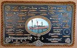
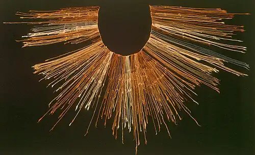
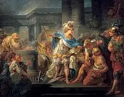
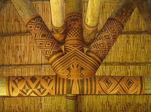
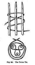
Knot board on Elbe 1 (ship, 1965)An example of a quipu from the Inca Empire, currently in the Larco Museum Collection.Alexander Cuts the Gordian Knot, by Jean-Simon Berthélemy (1743–1812)Gordian Knot statue (1990)Magimagi sennit of Fiji around wooden ceiling posts.Blackfoot “Teton” tipi tie[1]
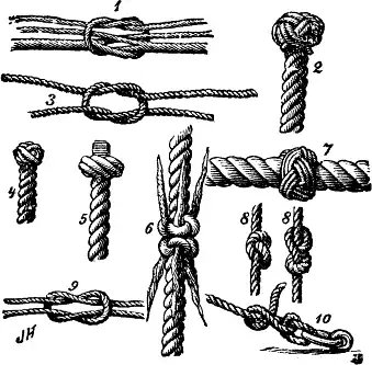
A knot is an intentional complication in cordage[2] which may be practical or decorative, or both. Practical knots are classified by function, including hitches, bends, loop knots, and splices: a hitch fastens a rope to another object; a bend fastens two ends of a rope to each another; a loop knot is any knot creating a loop; and splice denotes any multi-strand knot, including bends and loops.[3] A knot may also refer, in the strictest sense, to a stopper or knob at the end of a rope to keep that end from slipping through a grommet or eye.[4] Knots have excited interest since ancient times for their practical uses, as well as their topological intricacy, studied in the area of topology known as knot theory.
History
Knots and knotting have been used and studied throughout history. For example, Chinese knotting is a decorative handicraft art that began as a form of Chinese folk art in the Tang and Song dynasty (960–1279 AD) in China, later popularized in the Ming. Knot theory is the recent mathematical study of knots.
Knots of more recent origin include the friendship knot of Chinese knotting. The sheepshank knot originates from 1627[5] while the Western Union splice originates from the beginning of telegraphy.[6]
Use
There is a large variety of knots, each with properties that make it suitable for a range of tasks. Some knots are used to attach the rope (or other knotting material) to other objects such as another rope, cleat, ring, or stake. Some knots are used to bind or constrict objects. Decorative knots usually bind to themselves to produce attractive patterns.
Teaching
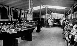
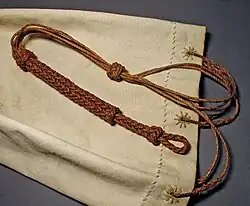
Sailors learning knots and ropework in the early 20th centurySailor bag with different knots
While some people can look at diagrams or photos and tie the illustrated knots, others learn best by watching how a knot is tied. Knot tying skills are often transmitted by sailors, scouts, climbers, canyoners, cavers, arborists, rescue professionals, stagehands, fishermen, linemen and surgeons. The International Guild of Knot Tyers is an organization dedicated to the promotion of knot tying.
Applications
Truckers in need of securing a load may use a trucker’s hitch, gaining mechanical advantage. Knots can save spelunkers from being buried under rock. Many knots can also be used as makeshift tools, for example, the bowline can be used as a rescue loop, and the munter hitch can be used for belaying. The diamond hitch was widely used to tie packages on to donkeys and mules.
In hazardous environments such as mountains, knots are very important. In the event of someone falling into a ravine or a similar terrain feature, with the correct equipment and knowledge of knots a rappel system can be set up to lower a rescuer down to a casualty and set up a hauling system to allow a third individual to pull both the rescuer and the casualty out of the ravine. Further application of knots includes developing a high line, which is similar to a zip line, and which can be used to move supplies, injured people, or the untrained across rivers, crevices, or ravines. Note the systems mentioned typically require carabiners and the use of multiple appropriate knots. These knots include the bowline, double figure eight, munter hitch, munter mule, prusik, autoblock, and clove hitch. Thus any individual who goes into a mountainous environment should have basic knowledge of knots and knot systems to increase safety and the ability to undertake activities such as rappelling.
Knots can be applied in combination to produce complex objects such as lanyards and netting. In ropework, the frayed end of a rope is held together by a type of knot called a whipping knot. Many types of textiles use knots to repair damage. Macramé, one kind of textile, is generated exclusively through the use of knotting, instead of knits, crochets, weaves or felting. Macramé can produce self-supporting three-dimensional textile structures, as well as flat work, and is often used ornamentally or decoratively.
Properties
Strength
Knots weaken the rope in which they are made.[7] When knotted rope is strained to its breaking point, it almost always fails at the knot or close to it, unless it is defective or damaged elsewhere. The bending, crushing, and chafing forces that hold a knot in place also unevenly stress rope fibers and ultimately lead to a reduction in strength. The exact mechanisms that cause the weakening and failure are complex and are the subject of continued study. Special fibers that show differences in color in response to strain are being developed and used to study stress as it relates to types of knots.[8][9]
Relative knot strength, also called knot efficiency, is the breaking strength of a knotted rope in proportion to the breaking strength of the rope without the knot. Determining a precise value for a particular knot is difficult because many factors can affect a knot efficiency test: the type of fiber, the style of rope, the size of rope, whether it is wet or dry, how the knot is dressed before loading, how rapidly it is loaded, whether the knot is repeatedly loaded, and so on. The efficiency of common knots ranges between 40 and 80% of the rope’s original strength.[10][11]
In most situations forming loops and bends with conventional knots is far more practical than using rope splices, even though the latter can maintain nearly the rope’s full strength. Prudent users allow for a large safety margin in the strength of rope chosen for a task due to the weakening effects of knots, aging, damage, shock loading, etc. The working load limit of a rope is generally specified with a significant safety factor, up to 15:1 for critical applications.[12] For life-threatening applications, other factors come into play.[13]
Security
Even if the rope does not break, a knot may still fail to hold. Knots that hold firm under a variety of adverse conditions are said to be more secure than those that do not.
The following sections describe the main ways that knots fail to hold.
Slipping
The load creates tension that pulls the rope back through the knot in the direction of the load. If this continues far enough, the working end passes into the knot and the knot unravels and fails. This behavior can worsen when the knot is repeatedly strained and let slack, dragged over rough terrain, or repeatedly struck against hard objects such as masts and flagpoles.
Even with secure knots, slippage may occur when the knot is first put under real tension. This can be mitigated by leaving plenty of rope at the working end outside of the knot, and by dressing the knot cleanly and tightening it as much as possible before loading. Sometimes, the use of a stopper knot or, even better, a backup knot can prevent the working end from passing through the knot; but if a knot is observed to slip, it is generally preferable to use a more secure knot. Life-critical applications often require backup knots to maximize safety.
To capsize a knot is to change its form and rearrange its parts, usually by pulling on specific ends in certain ways.[10] When used inappropriately, some knots tend to capsize easily or even spontaneously. Often the capsized form of the knot offers little resistance to slipping or spilling (coming untied). A reef knot, tying the binding of furled sails, can be capsized for untying by pulling on one tail and its standing part, which casts it into a cow hitch of the other half of the knot around the pulled strand.
Sometimes a knot is intentionally capsized as a method of tying another knot, as with the “lightning method” of tying a bowline. The carrick bend, is commonly shown to be tied by reeving a lattice form and then capsizing that into its stable form (in contrast to retaining the lattice form by seizing the tails to standing parts).
Sliding
In knots that are meant to grip other objects, failure can be defined as the knot moving relative to the gripped object. While the knot itself is not untied, it ceases to perform the desired function. For instance, a simple rolling hitch tied around a railing and pulled parallel to the railing might hold up to a certain tension, then start sliding. Sometimes this problem can be corrected by working-up the knot tighter before subjecting it to load, but usually the problem requires either a knot with more wraps or a rope of different diameter or material.
Releasability
Knots differ in the effort required to untie them after loading. Knots that are very difficult to untie, such as the water knot, are said to “jam” or be jamming knots. Knots that come untied with less difficulty, such as the Zeppelin bend, are referred to as “non-jamming“.
Components
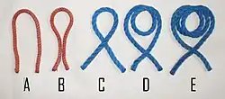
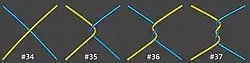
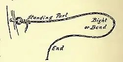
A: open loop, B: closed loop, C: turn, D: round turn, E: two round turns.#34 Cross #35 Elbow #36 Round turn#27 End #29 Bight #28 Standing
Bight
A bight is any curved section, slack part, or loop between the ends of a rope, string, or yarn.
Bitter end
As a ropeworker’s term, “bitter end” refers to the end of a rope that is tied off. In British nautical usage, the bitter end is the ship end of the anchor cable, secured by the anchor bitts and the bitter pin in the cable locker under the forecastle. At anchor, the more anchor line that is payed out, the better the anchor’s hold. In a storm, if the anchor drags, ships will pay out more and more anchor line until they reach the “bitter end.” At this point, they can only hope the anchor holds, hence the expression “hanging on to the bitter end”. (A bitt is a metal block with a crosspin for tying lines to, also found on piers.) Also, the working end.
Loop
A curve narrower than a bight but with separate ends.
Elbow
Two crossing points created by an extra twist in a loop or a circle.
Standing end
The standing end is the longer end of the rope not involved in the knot, often shown as unfinished. It is often (but not always) the end of the rope under load after the knot is complete. For example, when a clove hitch ties a boat to a pier, the end going to the boat is the standing end.
Standing part
Section of line between knot and the standing end (seen above).
Turn
A turn or single turn is a curve with crossed legs.
A round turn is the complete encirclement of an object; requires two passes.
Two round turns circles the object twice; requires three passes.
Working end
The active end of a line used in making the knot. May also be called the “running end”, “live end”, or “tag end”.
Working part
Section of line between knot and the working end.
Knot categories
The list of knots is extensive, but common properties allow for a useful system of categorization. For example, loop knots share the attribute of having some kind of an anchor point constructed on the standing end (such as a loop or overhand knot) into which the working end is easily hitched, using a round turn. An example of this is the bowline. Constricting knots often rely on friction to cinch down tight on loose bundles; an example is the Miller’s knot. Knots may belong to more than one category.
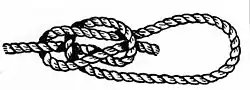
A knot tied with a hitch around one of its parts. In contrast, a loop is closed with a bend. While a slip knot can be closed, a loop remains the same size.
Some knots may be finished by passing a bight rather than the end, for ease of untying. The common shoelace knot is an example, being a reef knot with both ends slipped.
A binding knot used to prevent another line from fraying.
Basic useful knots
Alpine butterfly knot for a secure loop in the middle of a rope when the ends are not free
Bowline for tying a loop in the end of a rope, as around one’s waist or to secure a ring or grommet. The knot is also used as an anchor knot and is used in many knot systems that are used in mountainous terrain such as a highline or hauling system.
Constrictor knot for making bundles or cinching the neck of a sack, though this knot jams and may need to be cut
Trick knots are knots that are used as part of a magic trick, a joke, or a puzzle. They are useful for these purposes because they have a deceptive appearance, being easier or more difficult to tie or untie than their appearance would suggest. The easiest trick knot is the slip knot.[15] Other noted trick knots include:
Grief knot. The starkly differing behavior of the knot, depending on how it is arranged, has been exploited as the basis of a parlor trick.[16] When pulling on the standing ends the knot starts slipping and the working ends become crossed. By twisting the working ends so that they uncross and then recross in reverse, the knot’s structure capsizes so that it will no longer slip. The twisting motion resembles the turning of a key, “locking” and “unlocking” the knot.
Tom fool’s knot, used as a trick knot due to the speed with which it can be made.
Coxcombing
Coxcombing is a decorative knotwork performed by sailors during the Age of Sail.
The general purpose was to dress-up, protect, or help identify specific items and parts of ships and boats.
It is still found today in some whippings and wrappings of small diameter line on boat tillers and ships’ wheels to enhance the grip, or to identify rudder amidships.
Knot theory is a branch of topology.[17] It deals with the mathematical analysis of knots, their structure and properties, and with the relationships between different knots.[17] However, it does not take into account the role of friction in knots; in fact, no satisfactory general theory of knots that takes into account friction exists.[18]
In topology, a knot is a figure consisting of a single loop with any number of crossing or knotted elements: a closed curve in space which may be moved around so long as its strands never pass through each other. As a closed loop, a mathematical knot has no proper ends, and cannot be undone or untied; however, any physical knot in a piece of string can be thought of as a mathematical knot by fusing the two ends. A configuration of several knots winding around each other is called a link. Various mathematical techniques are used to classify and distinguish knots and links. For instance, the Alexander polynomial associates certain numbers with any given knot; these numbers are different for the trefoil knot, the figure-eight knot, and the unknot (a simple loop), showing that one cannot be moved into the other (without strands passing through each other).[17]
Physical theory of friction knots
A simple mathematical theory of hitches has been proposed by Bayman[19] and extended by Maddocks and Keller.[20] It makes predictions that are approximately correct when tested empirically.[18] No similarly successful theory has been developed for knots in general.
Knot tying consists of the techniques and skills employed in tying a knot in rope, nylon webbing, or other articles. The proper tying of a knot can be the difference between an attractive knot and a messy one, and occasionally life and death. It is important to understand the often subtle differences between what works, and what does not. For example, many knots “spill” or pull through, particularly if they are not “backed up,” usually with a single or double overhand knot to make sure the end of the rope does not make its way through the main knot, causing all strength to be lost.
Difficulty
The tying of a knot may be very straightforward (such as with an overhand knot), or it may be more complicated, such as a monkey’s fist knot. Tying knots correctly requires an understanding of the type of material being tied (string, cord, monofilament line, kernmantle rope, or nylon webbing). For example, cotton string may be very small and easy to tie with much internal friction to keep it from falling apart once tied, while stiff 5/8″ thick kernmantle rope will be very difficult to tie, and may be so slick as to tend to come apart once tied.
Material
The form of the material will influence the tying of a knot as well. Rope is round in cross-section, and has little dependence upon the manner in which the material is tied. Nylon webbing, on the other hand, is flat, and usually “tubular” in construction, meaning that it is spiral-woven, and has a hollow core. In order to retain as much of the strength as possible with webbing, the material must be tied “flat” such that parallel sections do not cross, and that the sections of webbing are not twisted when they cross each other within a knot.
The crossing of strands is important when dealing with round rope in other knots; for example, the figure-eight loop loses strength when strands are crossed while the knot is being “finished” and tightened. Moreover, the standing end or the end from which the hauling will be done must have the greater radius of curvature in the finished knot to maximize the strength of the knot.
Tools
Tools are sometimes employed in the finishing or untying of a knot, such as a fid, a tapered piece of wood that is often used in splicing. With the advent of wire rope, many other tools are used in the tying of “knots.” However, for cordage and other non-metallic appliances, the tools used are generally limited to sharp edges or blades such as a sheepsfoot blade, occasionally a fine needle for proper whipping of laid rope, a hot cutter for nylon and other synthetic fibers, and (for larger ropes) a shoe for smoothing out large knots by rolling them on the ground.
Use by animals
The hagfish is known to strip slime from its skin by tying itself into a simple overhand knot, and moving its body to make the knot travel toward the tail. It also uses this action in reverse (tail to head) to pry out flesh after biting into a carcass.[21]
↑Anthropological Papers of the American Museum of Natural History. Material culture of the Blackfoot Indians. 1910.
↑Ashley, Clifford W. (1944), The Ashley Book of Knots, New York: Doubleday, p.12, The word knot has three distinct meanings in common use. In the broadest sense it applies to all complications in cordage, except accidental ones, such as snarls and kinks, and complications adapted for storage, such as coils, hanks, skeins, balls, etc.
↑Ashley, Clifford W. (1944), The Ashley Book of Knots, New York: Doubleday, p.12
↑Ashley, Clifford W. (1944), The Ashley Book of Knots, New York: Doubleday, p.12, In its second sense it does not include bends, hitches, splices, and sinnets, and in its third and narrowest sense the term applies only to a knob tied in a rope to prevent unreeving, to provide a handhold, or (in small material only) to prevent fraying.
↑Turner, John C.; Griend, Pieter Van De; Warner, Charles (1996-05-30). History And Science Of Knots. World Scientific. ISBN978-981-4499-64-4.
↑Sharp, John MacLaren (1915). Practical Electric Wiring. New York and London: D. Appleton and Company. pp.12–14.
12Warner, Charles (1996), “Studies on the Behaviour of Knots”, in Turner, J.C.; van de Griend, P. (eds.), History and Science of Knots, K&E Series on Knots and Everything, vol.11, Singapore: World Scientific Publishing, pp.181–203, ISBN978-981-02-2469-1
This article is adapted from “Knot” on Wikipedia, written by its contributors, and used under CC BY-SA 4.0. Text on this page is available under the same licence. Source snapshot: Wikipedia via Kiwix, 2026-07-20.
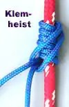
The klemheist knot or French Machard knot is a type of friction hitch that grips the rope when weight is applied, and is free to move when the weight is released. It is used similarly to a Prusik knot or the Bachmann knot to ascend or descend a climbing rope. One advantage is that webbing can be used as an alternative to cord. The Klemheist is easier to slide up than a Prusik. The klemheist is also a way to attach a snubber to the anchor rope of small boats, with the advantage that it is easy to undo.[1]
Sometimes the knot name is misspelled as “kleimheist”, with an extra “i”.
Technique
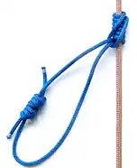
Klemheist knot with loop
Make a secure loop of a cord (see Double fisherman’s knot) that is definitely narrower than the rope. Wrap from one end around the rope two or three times in a direction that will be down. The loose end is then threaded through the starting end, and carefully tightened to leave the wraps neat. In use, strain must be taken only on the hanging end. If the knot slips when load is placed on the hanging loop, re-tie around the climbing rope another time or two, until there is no slippage. Holding around the wraps will let you slide the knot up or down. Making the wraps slide when the hitch is under tension will create friction heat on the rope and the knot.
This article is adapted from “Klemheist knot” on Wikipedia, written by its contributors, and used under CC BY-SA 4.0. Text on this page is available under the same licence. Source snapshot: Wikipedia via Kiwix, 2026-07-20.
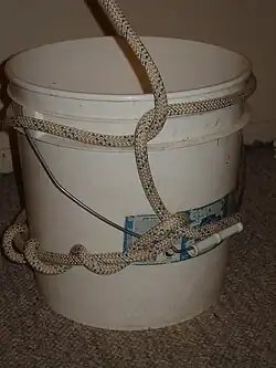
The killick hitch/ˈkɪlɪk/ is a type of hitch knot used to attach a rope to oddly shaped objects.[1]:32 It is a combination of a timber hitch tied in conjunction with a half hitch [1]:23 which is added to lend support and stability when pulling or hoisting the object.[2]
A killick is “a small anchor or weight for mooring a boat, sometimes consisting of a stone secured by pieces of wood”.[3]
Use
The killick hitch is used to anchor small boats, usually by using some odd shaped heavy object. It is used by oystermen because the anchor is more readily moved than with other methods.
This article is adapted from “Killick hitch” on Wikipedia, written by its contributors, and used under CC BY-SA 4.0. Text on this page is available under the same licence. Source snapshot: Wikipedia via Kiwix, 2026-07-20.
The pictures represent the L polynomial of the diagrams which differ inside a disc as shown but are identical outside.
Kauffman showed that L exists and is a regular isotopy invariant of unoriented links. It follows easily that F is an ambient isotopy invariant of oriented links.
The Jones polynomial is a special case of the Kauffman polynomial, as the L polynomial specializes to the bracket polynomial. The Kauffman polynomial is related to Chern–Simons gauge theories for SO(N) in the same way that the HOMFLY polynomial is related to Chern–Simons gauge theories for SU(N).[2]
This article is adapted from “Kauffman polynomial” on Wikipedia, written by its contributors, and used under CC BY-SA 4.0. Text on this page is available under the same licence. Source snapshot: Wikipedia via Kiwix, 2026-07-20.
The Kalmyk loop (Russian: калмыцкий узел) is a fixed loop still largely unused in the West, but common in Russia and often used instead of the bowline.
The knot is named after the Kalmyks, a nomad ethnicity in Russia.
It is very quick to tie, it is secure, and it undoes quickly when pulling the free end.
The knot is not mentioned in The Ashley Book of Knots but is found in its Russian equivalent, the book “Морские узлы” by Lev Skryagin.
Without the slip, the knot is known as the Eskimo bowline or Cossack knot.
Sources
Скрягин Л. Н. Морские узлы — Москва, Транспорт, 1982
This article is adapted from “Kalmyk loop” on Wikipedia, written by its contributors, and used under CC BY-SA 4.0. Text on this page is available under the same licence. Source snapshot: Wikipedia via Kiwix, 2026-07-20.


 (Unknot)
 (Trefoil Knot)



 (Figure-eight Knot)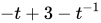



 (Cinquefoil Knot)



 (Granny Knot)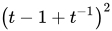


 (Square Knot)


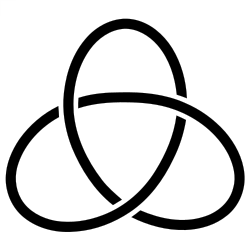 The left-trefoil knot.
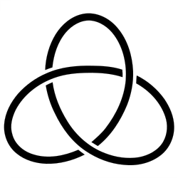 The right-trefoil knot.
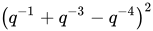
 is the product of knots in knot polynomials.