Category: Knots

  • Blackwall hitch

    Blackwall hitch
    Blackwall hitch
    Category Hitch
    Related Half hitch
    Releasing Non-jamming
    Typical use To temporarily attach a rope to a hook when they both are of equal size.
    Caveat Likely to slip if subjected to more than ordinary strain
    ABoK #1875

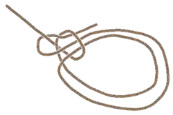
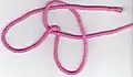
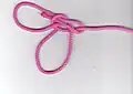
    The blackwall hitch is a temporary means of attaching a rope to a hook. Made of a simple half hitch over the hook, it will only hold when subjected to constant tension. It is used when the rope and hook are of equal size, but it is likely to slip if subjected to more than ordinary tension. Human life should never be trusted to it.[1]

    See also

    References

    1. “Blackwall Hitch”. Archived from the original on August 6, 2002.

    This article is adapted from “Blackwall hitch” on Wikipedia, written by its contributors, and used under CC BY-SA 4.0. Text on this page is available under the same licence. Source snapshot: Wikipedia via Kiwix, 2026-07-20.

  • Pretzel link

    Pretzel link
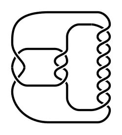
    The (−2,3,7) pretzel knot has two right-handed twists in its first tangle, three left-handed twists in its second, and seven left-handed twists in its third.
    Pretzel link
    P(5,3,-2) = T(5,3) = 10124
    Pretzel link
    P(3,3,-2) = T(4,3) = 819
    Only two knots are both torus and pretzel[1]

    In the mathematical theory of knots, a pretzel link is a special kind of link. It consists of a finite number of tangles made of two intertwined circular helices. The tangles are connected cyclicly,[2] and the first component of the first tangle is connected to the second component of the second tangle, the first component of the second tangle is connected to the second component of the third tangle, and so on. Finally, the first component of the last tangle is connected to the second component of the first. A pretzel link which is also a knot (that is, a link with one component) is a pretzel knot.

    Each tangle is characterized by its number of twists: positive if they are counter-clockwise or left-handed, negative if clockwise or right-handed. In the standard projection of the ( p 1 , p 2 , , p n ) {\displaystyle (p_{1},\,p_{2},\dots ,\,p_{n})} {\displaystyle (p_{1},\,p_{2},\dots ,\,p_{n})} pretzel link, there are p 1 {\displaystyle p_{1}} {\displaystyle p_{1}}left-handed crossings in the first tangle, p 2 {\displaystyle p_{2}} {\displaystyle p_{2}}in the second, and, in general, p n {\displaystyle p_{n}} {\displaystyle p_{n}}in the nth.

    A pretzel link can also be described as a Montesinos link with integer tangles.

    Some basic results

    The ( p 1 , p 2 , , p n ) {\displaystyle (p_{1},p_{2},\dots ,p_{n})} {\displaystyle (p_{1},p_{2},\dots ,p_{n})} pretzel link is a knot iff both n {\displaystyle n} {\displaystyle n} and all the p i {\displaystyle p_{i}} {\displaystyle p_{i}} are odd or exactly one of the p i {\displaystyle p_{i}} {\displaystyle p_{i}} is even.[3]

    The ( p 1 , p 2 , , p n ) {\displaystyle (p_{1},\,p_{2},\dots ,\,p_{n})} {\displaystyle (p_{1},\,p_{2},\dots ,\,p_{n})} pretzel link is split if at least two of the p i {\displaystyle p_{i}} {\displaystyle p_{i}} are zero; but the converse is false.

    The ( p 1 , p 2 , , p n ) {\displaystyle (-p_{1},-p_{2},\dots ,-p_{n})} {\displaystyle (-p_{1},-p_{2},\dots ,-p_{n})} pretzel link is the mirror image of the ( p 1 , p 2 , , p n ) {\displaystyle (p_{1},\,p_{2},\dots ,\,p_{n})} {\displaystyle (p_{1},\,p_{2},\dots ,\,p_{n})} pretzel link.

    The ( p 1 , p 2 , , p n ) {\displaystyle (p_{1},\,p_{2},\dots ,\,p_{n})} {\displaystyle (p_{1},\,p_{2},\dots ,\,p_{n})} pretzel link is isotopic to the ( p 2 , p 3 , , p n , p 1 ) {\displaystyle (p_{2},\,p_{3},\dots ,\,p_{n},\,p_{1})} {\displaystyle (p_{2},\,p_{3},\dots ,\,p_{n},\,p_{1})} pretzel link. Thus, too, the ( p 1 , p 2 , , p n ) {\displaystyle (p_{1},\,p_{2},\dots ,\,p_{n})} {\displaystyle (p_{1},\,p_{2},\dots ,\,p_{n})} pretzel link is isotopic to the ( p k , p k + 1 , , p n , p 1 , p 2 , , p k 1 ) {\displaystyle (p_{k},\,p_{k+1},\dots ,\,p_{n},\,p_{1},\,p_{2},\dots ,\,p_{k-1})} {\displaystyle (p_{k},\,p_{k+1},\dots ,\,p_{n},\,p_{1},\,p_{2},\dots ,\,p_{k-1})} pretzel link.[3]

    The ( p 1 , p 2 , , p n ) {\displaystyle (p_{1},\,p_{2},\,\dots ,\,p_{n})} {\displaystyle (p_{1},\,p_{2},\,\dots ,\,p_{n})} pretzel link is isotopic to the ( p n , p n 1 , , p 2 , p 1 ) {\displaystyle (p_{n},\,p_{n-1},\dots ,\,p_{2},\,p_{1})} {\displaystyle (p_{n},\,p_{n-1},\dots ,\,p_{2},\,p_{1})} pretzel link. However, if one orients the links in a canonical way, then these two links have opposite orientations.

    Some examples

    The (1, 1, 1) pretzel knot is the (right-handed) trefoil; the (−1, −1, −1) pretzel knot is its mirror image.

    The (5, −1, −1) pretzel knot is the stevedore knot (61).

    If p, q, r are distinct odd integers greater than 1, then the (p, q, r) pretzel knot is a non-invertible knot.

    The (2p, 2q, 2r) pretzel link is a link formed by three linked unknots.

    The (−3, 0, −3) pretzel knot (square knot (mathematics)) is the connected sum of two trefoil knots.

    The (0, q, 0) pretzel link is the split union of an unknot and another knot.

    Montesinos

    A Montesinos link is a special kind of link that generalizes pretzel links (a pretzel link can also be described as a Montesinos link with integer tangles). A Montesinos link which is also a knot (i.e., a link with one component) is a Montesinos knot.

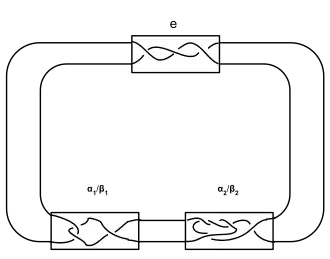
    A Montesinos link is composed of several rational tangles. One notation for a Montesinos link is K ( e ; α 1 / β 1 , α 2 / β 2 , , α n / β n ) {\displaystyle K(e;\alpha _{1}/\beta _{1},\alpha _{2}/\beta _{2},\ldots ,\alpha _{n}/\beta _{n})} {\displaystyle K(e;\alpha _{1}/\beta _{1},\alpha _{2}/\beta _{2},\ldots ,\alpha _{n}/\beta _{n})}.[4]

    In this notation, e {\displaystyle e} {\displaystyle e} and all the α i {\displaystyle \alpha _{i}} {\displaystyle \alpha _{i}} and β i {\displaystyle \beta _{i}} {\displaystyle \beta _{i}} are integers. The Montesinos link given by this notation consists of the sum of the rational tangles given by the integer e {\displaystyle e} {\displaystyle e} and the rational tangles α 1 / β 1 , α 2 / β 2 , , α n / β n {\displaystyle \alpha _{1}/\beta _{1},\alpha _{2}/\beta _{2},\ldots ,\alpha _{n}/\beta _{n}} {\displaystyle \alpha _{1}/\beta _{1},\alpha _{2}/\beta _{2},\ldots ,\alpha _{n}/\beta _{n}}

    These knots and links are named after the Spanish topologist José María Montesinos Amilibia, who first introduced them in 1973.[5]

    Utility

    (−2, 3, 2n + 1) pretzel links are especially useful in the study of 3-manifolds. Many results have been stated about the manifolds that result from Dehn surgery on the (−2,3,7) pretzel knot in particular.

    The hyperbolic volume of the complement of the (−2,3,8) pretzel link is 4 times Catalan’s constant, approximately 3.66. This pretzel link complement is one of two two-cusped hyperbolic manifolds with the minimum possible volume, the other being the complement of the Whitehead link.[6]

    Link diagram showing a Montesinos link
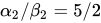
    A Montesinos link. In this example, e = 3 {\displaystyle e=-3} {\displaystyle e=-3} , α 1 / β 1 = 3 / 2 {\displaystyle \alpha _{1}/\beta _{1}=-3/2} {\displaystyle \alpha _{1}/\beta _{1}=-3/2} and α 2 / β 2 = 5 / 2 {\displaystyle \alpha _{2}/\beta _{2}=5/2} {\displaystyle \alpha _{2}/\beta _{2}=5/2}.
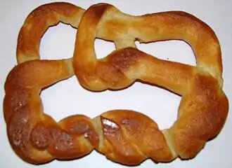
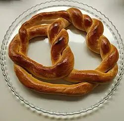
    A pretzel baked in the shape of a (–2,3,7) pretzel knot
    Edible (−2,3,7) pretzel knot
    A pretzel baked in the shape of a (–2,3,7) pretzel knot, with shiny egg glaze
    Another edible (–2,3,7) pretzel knot, glazed to near perfection

    References

    1. 10 124“, The Knot Atlas. Accessed November 19, 2017.
    2. Pretzel link at Mathcurve
    3. 1 2 Kawauchi, Akio (1996). A survey of knot theory. Birkhäuser. ISBN 3-7643-5124-1
    4. Zieschang, Heiner (1984), “Classification of Montesinos knots”, Topology (Leningrad, 1982), Lecture Notes in Mathematics, vol. 1060, Berlin: Springer, pp. 378–389, doi:10.1007/BFb0099953, MR 0770257
    5. Montesinos, José M. (1973), “Seifert manifolds that are ramified two-sheeted cyclic coverings”, Boletín de la Sociedad Matemática Mexicana, 2, 18: 1–32, MR 0341467
    6. Agol, Ian (2010), “The minimal volume orientable hyperbolic 2-cusped 3-manifolds”, Proceedings of the American Mathematical Society, 138 (10): 3723–3732, arXiv:0804.0043, doi:10.1090/S0002-9939-10-10364-5, MR 2661571.

    Further reading

    • Trotter, Hale F.: Non-invertible knots exist, Topology, 2 (1963), 272–280.
    • Burde, Gerhard; Zieschang, Heiner (2003). Knots. De Gruyter studies in mathematics. Vol. 5 (2nd revised and extended ed.). Walter de Gruyter. ISBN 3110170051. ISSN 0179-0986. Zbl 1009.57003.

    This article is adapted from “Pretzel link” on Wikipedia, written by its contributors, and used under CC BY-SA 4.0. Text on this page is available under the same licence. Source snapshot: Wikipedia via Kiwix, 2026-07-20.

  • Birman–Wenzl algebra

    In mathematics, the Birman–Murakami–Wenzl (BMW) algebra, introduced by Joan Birman and Hans Wenzl (1989) and Jun Murakami (1987), is a two-parameter family of algebras C n ( , m ) {\displaystyle \mathrm {C} _{n}(\ell ,m)} {\displaystyle \mathrm {C} _{n}(\ell ,m)} of dimension 1 3 5 ( 2 n 1 ) {\displaystyle 1\cdot 3\cdot 5\cdots (2n-1)} {\displaystyle 1\cdot 3\cdot 5\cdots (2n-1)} having the Hecke algebra of the symmetric group as a quotient. It is related to the Kauffman polynomial of a link. It is a deformation of the Brauer algebra in much the same way that Hecke algebras are deformations of the group algebra of the symmetric group.

    Definition

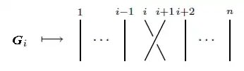
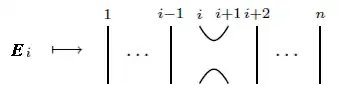
    For each natural number n, the BMW algebra C n ( , m ) {\displaystyle \mathrm {C} _{n}(\ell ,m)} {\displaystyle \mathrm {C} _{n}(\ell ,m)} is generated by G 1 ± 1 , G 2 ± 1 , , G n 1 ± 1 , E 1 , E 2 , , E n 1 {\displaystyle G_{1}^{\pm 1},G_{2}^{\pm 1},\dots ,G_{n-1}^{\pm 1},E_{1},E_{2},\dots ,E_{n-1}} {\displaystyle G_{1}^{\pm 1},G_{2}^{\pm 1},\dots ,G_{n-1}^{\pm 1},E_{1},E_{2},\dots ,E_{n-1}} and relations:

    G i G j = G j G i , i f | i j | 2 , {\displaystyle G_{i}G_{j}=G_{j}G_{i},\mathrm {if} \left\vert i-j\right\vert \geq 2,} {\displaystyle G_{i}G_{j}=G_{j}G_{i},\mathrm {if} \left\vert i-j\right\vert \geq 2,}
    G i G i + 1 G i = G i + 1 G i G i + 1 , {\displaystyle G_{i}G_{i+1}G_{i}=G_{i+1}G_{i}G_{i+1},} {\displaystyle G_{i}G_{i+1}G_{i}=G_{i+1}G_{i}G_{i+1},}         E i E i ± 1 E i = E i , {\displaystyle E_{i}E_{i\pm 1}E_{i}=E_{i},} {\displaystyle E_{i}E_{i\pm 1}E_{i}=E_{i},}
    G i + G i 1 = m ( 1 + E i ) , {\displaystyle G_{i}+{G_{i}}^{-1}=m(1+E_{i}),} {\displaystyle G_{i}+{G_{i}}^{-1}=m(1+E_{i}),}
    G i ± 1 G i E i ± 1 = E i G i ± 1 G i = E i E i ± 1 , {\displaystyle G_{i\pm 1}G_{i}E_{i\pm 1}=E_{i}G_{i\pm 1}G_{i}=E_{i}E_{i\pm 1},} {\displaystyle G_{i\pm 1}G_{i}E_{i\pm 1}=E_{i}G_{i\pm 1}G_{i}=E_{i}E_{i\pm 1},}      G i ± 1 E i G i ± 1 = G i 1 E i ± 1 G i 1 , {\displaystyle G_{i\pm 1}E_{i}G_{i\pm 1}={G_{i}}^{-1}E_{i\pm 1}{G_{i}}^{-1},} {\displaystyle G_{i\pm 1}E_{i}G_{i\pm 1}={G_{i}}^{-1}E_{i\pm 1}{G_{i}}^{-1},}
    G i ± 1 E i E i ± 1 = G i 1 E i ± 1 , {\displaystyle G_{i\pm 1}E_{i}E_{i\pm 1}={G_{i}}^{-1}E_{i\pm 1},} {\displaystyle G_{i\pm 1}E_{i}E_{i\pm 1}={G_{i}}^{-1}E_{i\pm 1},}      E i ± 1 E i G i ± 1 = E i ± 1 G i 1 , {\displaystyle E_{i\pm 1}E_{i}G_{i\pm 1}=E_{i\pm 1}{G_{i}}^{-1},} {\displaystyle E_{i\pm 1}E_{i}G_{i\pm 1}=E_{i\pm 1}{G_{i}}^{-1},}
    G i E i = E i G i = l 1 E i , {\displaystyle G_{i}E_{i}=E_{i}G_{i}=l^{-1}E_{i},} {\displaystyle G_{i}E_{i}=E_{i}G_{i}=l^{-1}E_{i},}      E i G i ± 1 E i = l E i . {\displaystyle E_{i}G_{i\pm 1}E_{i}=lE_{i}.} {\displaystyle E_{i}G_{i\pm 1}E_{i}=lE_{i}.}

    These relations imply the further relations:

    E i E j = E j E i , i f | i j | 2 , {\displaystyle E_{i}E_{j}=E_{j}E_{i},\mathrm {if} \left\vert i-j\right\vert \geq 2,} {\displaystyle E_{i}E_{j}=E_{j}E_{i},\mathrm {if} \left\vert i-j\right\vert \geq 2,}
    ( E i ) 2 = ( m 1 ( l + l 1 ) 1 ) E i , {\displaystyle (E_{i})^{2}=(m^{-1}(l+l^{-1})-1)E_{i},} {\displaystyle (E_{i})^{2}=(m^{-1}(l+l^{-1})-1)E_{i},}
    G i 2 = m ( G i + l 1 E i ) 1. {\displaystyle {G_{i}}^{2}=m(G_{i}+l^{-1}E_{i})-1.} {\displaystyle {G_{i}}^{2}=m(G_{i}+l^{-1}E_{i})-1.}

    This is the original definition given by Birman and Wenzl. However a slight change by the introduction of some minus signs is sometimes made, in accordance with Kauffman’s ‘Dubrovnik’ version of his link invariant. In that way, the fourth relation in Birman & Wenzl’s original version is changed to

    1. (Kauffman skein relation)
      G i G i 1 = m ( 1 E i ) , {\displaystyle G_{i}-{G_{i}}^{-1}=m(1-E_{i}),} {\displaystyle G_{i}-{G_{i}}^{-1}=m(1-E_{i}),}

    Given invertibility of m, the rest of the relations in Birman & Wenzl’s original version can be reduced to

    1. (Idempotent relation)
      ( E i ) 2 = ( m 1 ( l l 1 ) + 1 ) E i , {\displaystyle (E_{i})^{2}=(m^{-1}(l-l^{-1})+1)E_{i},} {\displaystyle (E_{i})^{2}=(m^{-1}(l-l^{-1})+1)E_{i},}
    2. (Braid relations)
      G i G j = G j G i , if  | i j | 2 ,  and  G i G i + 1 G i = G i + 1 G i G i + 1 , {\displaystyle G_{i}G_{j}=G_{j}G_{i},{\text{if }}\left\vert i-j\right\vert \geqslant 2,{\text{ and }}G_{i}G_{i+1}G_{i}=G_{i+1}G_{i}G_{i+1},} {\displaystyle G_{i}G_{j}=G_{j}G_{i},{\text{if }}\left\vert i-j\right\vert \geqslant 2,{\text{ and }}G_{i}G_{i+1}G_{i}=G_{i+1}G_{i}G_{i+1},}
    3. (Tangle relations)
      E i E i ± 1 E i = E i  and  G i G i ± 1 E i = E i ± 1 E i , {\displaystyle E_{i}E_{i\pm 1}E_{i}=E_{i}{\text{ and }}G_{i}G_{i\pm 1}E_{i}=E_{i\pm 1}E_{i},} {\displaystyle E_{i}E_{i\pm 1}E_{i}=E_{i}{\text{ and }}G_{i}G_{i\pm 1}E_{i}=E_{i\pm 1}E_{i},}
    4. (Delooping relations)
      G i E i = E i G i = l 1 E i  and  E i G i ± 1 E i = l E i . {\displaystyle G_{i}E_{i}=E_{i}G_{i}=l^{-1}E_{i}{\text{ and }}E_{i}G_{i\pm 1}E_{i}=lE_{i}.} {\displaystyle G_{i}E_{i}=E_{i}G_{i}=l^{-1}E_{i}{\text{ and }}E_{i}G_{i\pm 1}E_{i}=lE_{i}.}

    Properties

    • The dimension of C n ( , m ) {\displaystyle \mathrm {C} _{n}(\ell ,m)} {\displaystyle \mathrm {C} _{n}(\ell ,m)} is ( 2 n ) ! / ( 2 n n ! ) {\displaystyle (2n)!/(2^{n}n!)} {\displaystyle (2n)!/(2^{n}n!)}.
    • The Iwahori–Hecke algebra associated with the symmetric group S n {\displaystyle S_{n}} {\displaystyle S_{n}} is a quotient of the Birman–Murakami–Wenzl algebra C n {\displaystyle \mathrm {C} _{n}} {\displaystyle \mathrm {C} _{n}}.
    • The Artin braid group embeds in the BMW algebra: B n C n {\displaystyle B_{n}\hookrightarrow \mathrm {C} _{n}} {\displaystyle B_{n}\hookrightarrow \mathrm {C} _{n}}.

    Isomorphism between the BMW algebras and Kauffman’s tangle algebras

    It is proved by Morton & Wassermann (1989) that the BMW algebra C n ( , m ) {\displaystyle \mathrm {C} _{n}(\ell ,m)} {\displaystyle \mathrm {C} _{n}(\ell ,m)} is isomorphic to the Kauffman’s tangle algebra K T n {\displaystyle \mathrm {KT} _{n}} {\displaystyle \mathrm {KT} _{n}}. The isomorphism ϕ : C n K T n {\displaystyle \phi \colon \mathrm {C} _{n}\to \mathrm {KT} _{n}} {\displaystyle \phi \colon \mathrm {C} _{n}\to \mathrm {KT} _{n}} is defined by
    Birman–Wenzl algebra and Birman–Wenzl algebra

    Baxterisation of Birman–Murakami–Wenzl algebra

    Define the face operator as

    U i ( u ) = 1 i sin u sin λ sin μ ( e i ( u λ ) G i e i ( u λ ) G i 1 ) {\displaystyle U_{i}(u)=1-{\frac {i\sin u}{\sin \lambda \sin \mu }}(e^{i(u-\lambda )}G_{i}-e^{-i(u-\lambda )}{G_{i}}^{-1})} {\displaystyle U_{i}(u)=1-{\frac {i\sin u}{\sin \lambda \sin \mu }}(e^{i(u-\lambda )}G_{i}-e^{-i(u-\lambda )}{G_{i}}^{-1})},

    where λ {\displaystyle \lambda } {\displaystyle \lambda } and μ {\displaystyle \mu } {\displaystyle \mu } are determined by

    2 cos λ = 1 + ( l l 1 ) / m {\displaystyle 2\cos \lambda =1+(l-l^{-1})/m} {\displaystyle 2\cos \lambda =1+(l-l^{-1})/m}

    and

    2 cos λ = 1 + ( l l 1 ) / ( λ sin μ ) {\displaystyle 2\cos \lambda =1+(l-l^{-1})/(\lambda \sin \mu )} {\displaystyle 2\cos \lambda =1+(l-l^{-1})/(\lambda \sin \mu )}.

    Then the face operator satisfies the Yang–Baxter equation.

    U i + 1 ( v ) U i ( u + v ) U i + 1 ( u ) = U i ( u ) U i + 1 ( u + v ) U i ( v ) {\displaystyle U_{i+1}(v)U_{i}(u+v)U_{i+1}(u)=U_{i}(u)U_{i+1}(u+v)U_{i}(v)} {\displaystyle U_{i+1}(v)U_{i}(u+v)U_{i+1}(u)=U_{i}(u)U_{i+1}(u+v)U_{i}(v)}

    Now E i = U i ( λ ) {\displaystyle E_{i}=U_{i}(\lambda )} {\displaystyle E_{i}=U_{i}(\lambda )} with

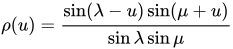
    ρ ( u ) = sin ( λ u ) sin ( μ + u ) sin λ sin μ {\displaystyle \rho (u)={\frac {\sin(\lambda -u)\sin(\mu +u)}{\sin \lambda \sin \mu }}} {\displaystyle \rho (u)={\frac {\sin(\lambda -u)\sin(\mu +u)}{\sin \lambda \sin \mu }}}.

    In the limits u ± i {\displaystyle u\to \pm i\infty } {\displaystyle u\to \pm i\infty }, the braids G j ± {\displaystyle {G_{j}}^{\pm }} {\displaystyle {G_{j}}^{\pm }} can be recovered up to a scale factor.

    History

    In 1984, Vaughan Jones introduced a new polynomial invariant of link isotopy types which is called the Jones polynomial. The invariants are related to the traces of irreducible representations of Hecke algebras associated with the symmetric groups. Murakami (1987) showed that the Kauffman polynomial can also be interpreted as a function F {\displaystyle F} {\displaystyle F} on a certain associative algebra. In 1989, Birman & Wenzl (1989) constructed a two-parameter family of algebras C n ( , m ) {\displaystyle \mathrm {C} _{n}(\ell ,m)} {\displaystyle \mathrm {C} _{n}(\ell ,m)} with the Kauffman polynomial K n ( , m ) {\displaystyle K_{n}(\ell ,m)} {\displaystyle K_{n}(\ell ,m)} as trace after appropriate renormalization.

    References


    This article is adapted from “Birman–Wenzl algebra” on Wikipedia, written by its contributors, and used under CC BY-SA 4.0. Text on this page is available under the same licence. Source snapshot: Wikipedia via Kiwix, 2026-07-20.

  • Pratt knot

    Pratt knot
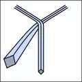
    A blue Pratt knot.

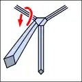
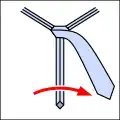
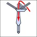
    The Pratt knot is a method of tying a necktie. It is also known as the Shelby knot.[1][2][3] The knot was created in the late 1950s by Jerry Pratt, an employee of the US Chamber of Commerce.[4] It was popularized as the Shelby knot after then 92-year-old Pratt taught it in 1986 to television reporter Don Shelby, who he felt had been tying his tie poorly on the air.[5] Shelby then refined the Pratt knot with local clothier Kingford Bavender and wore it on the air with a spread collar where it stood out and attracted attention for its symmetry and trim precision.[6]

    The knot is a variation on the Nicky knot. Both the Pratt and Nicky knots are tied inside out, though only the Nicky knot is self-releasing. Before its popularization in a 1989 New York Times article, the knot was unknown within the fashion world and not recorded in the tie industry’s standard reference guide of the time, Getting Knotted – 188 Knots for Necks by Davide Mosconi and Riccardo Villarosa in Milan, Italy.[6][7]

    The Pratt knot uses less length than the half-Windsor or Windsor knots, and so is well suited to shorter ties or taller men. Unlike the four-in-hand knot, the Pratt method produces a symmetrical knot. It is of medium thickness.

    Using notation from and according to The 85 Ways to Tie a Tie, the knot is tied

    • Lo Ci Lo Ri Co T (knot 5).
    • Pratt knot
    • Pratt knot
    • Pratt knot
    • Pratt knot

    See also

    References

    External links


    This article is adapted from “Pratt knot” on Wikipedia, written by its contributors, and used under CC BY-SA 4.0. Text on this page is available under the same licence. Source snapshot: Wikipedia via Kiwix, 2026-07-20.

  • Biracks and biquandles

    In mathematics, biquandles and biracks are sets with binary operations that generalize quandles and racks. In the theory of virtual knots, biquandles are analagous to quandles in the theory of classical knots. Biracks and racks have the same relation, while a biquandle is a birack which satisfies some additional conditions.

    Definitions

    A birack is a set X {\displaystyle X} {\displaystyle X}, two right-invertible operations _ {\displaystyle {\underline {\triangleright }}} {\displaystyle {\underline {\triangleright }}} , ¯ {\displaystyle ,{\overline {\triangleright }}} {\displaystyle ,{\overline {\triangleright }}} and a bijection π : X X {\displaystyle \pi \colon X\to X} {\displaystyle \pi \colon X\to X} such that for all a , b , c X {\displaystyle a,b,c\in X} {\displaystyle a,b,c\in X},

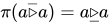
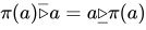
    1. π ( a ¯ a ) = a _ a {\textstyle \pi (a{\overline {\triangleright }}a)=a{\underline {\triangleright }}a} {\textstyle \pi (a{\overline {\triangleright }}a)=a{\underline {\triangleright }}a} and π ( a ) ¯ a = a _ π ( a ) {\displaystyle \pi (a){\overline {\triangleright }}a=a{\underline {\triangleright }}\pi (a)} {\displaystyle \pi (a){\overline {\triangleright }}a=a{\underline {\triangleright }}\pi (a)}.

    2. The map H : X × X X × X {\displaystyle H\colon X\times X\to X\times X} {\displaystyle H\colon X\times X\to X\times X} defined by H ( a , b ) = ( b ¯ a , a _ b ) {\displaystyle H(a,b)=(b{\overline {\triangleright }}a,a{\underline {\triangleright }}b)} {\displaystyle H(a,b)=(b{\overline {\triangleright }}a,a{\underline {\triangleright }}b)} is invertible.

    3. The exchange laws

    • ( a _ b ) _ ( c _ b ) = ( a _ c ) _ ( b ¯ c ) {\displaystyle (a{\underline {\triangleright }}b){\underline {\triangleright }}(c{\underline {\triangleright }}b)=(a{\underline {\triangleright }}c){\underline {\triangleright }}(b{\overline {\triangleright }}c)} {\displaystyle (a{\underline {\triangleright }}b){\underline {\triangleright }}(c{\underline {\triangleright }}b)=(a{\underline {\triangleright }}c){\underline {\triangleright }}(b{\overline {\triangleright }}c)}
    • ( a _ b ) ¯ ( c _ b ) = ( a ¯ c ) _ ( b ¯ c ) {\displaystyle (a{\underline {\triangleright }}b){\overline {\triangleright }}(c{\underline {\triangleright }}b)=(a{\overline {\triangleright }}c){\underline {\triangleright }}(b{\overline {\triangleright }}c)} {\displaystyle (a{\underline {\triangleright }}b){\overline {\triangleright }}(c{\underline {\triangleright }}b)=(a{\overline {\triangleright }}c){\underline {\triangleright }}(b{\overline {\triangleright }}c)}
    • ( a ¯ b ) ¯ ( c ¯ b ) = ( a ¯ c ) ¯ ( b _ c ) {\displaystyle (a{\overline {\triangleright }}b){\overline {\triangleright }}(c{\overline {\triangleright }}b)=(a{\overline {\triangleright }}c){\overline {\triangleright }}(b{\underline {\triangleright }}c)} {\displaystyle (a{\overline {\triangleright }}b){\overline {\triangleright }}(c{\overline {\triangleright }}b)=(a{\overline {\triangleright }}c){\overline {\triangleright }}(b{\underline {\triangleright }}c)}.

    If π = i d {\textstyle \pi =id} {\textstyle \pi =id} is the identity map, X {\textstyle X} {\textstyle X} is called a biquandle.[1]

    Biracks and biquandles were first introduced by Roger Fenn, Mercedes Jordan-Santana and Louis Kauffman in 2004.[2]

    Note that the three conditions above correspond directly to the three Reidemeister moves in knot therory, showing the close connections between knots and biracks.[3]

    Examples

    Let X {\textstyle X} {\textstyle X} be a set with two bijection σ , τ : X X {\displaystyle \sigma ,\tau \colon X\to X} {\displaystyle \sigma ,\tau \colon X\to X} that commute. Then the constant action birack is defined by a _ b = σ ( a ) {\displaystyle a{\underline {\triangleright }}b=\sigma (a)} {\displaystyle a{\underline {\triangleright }}b=\sigma (a)} and a ¯ b = τ ( x ) {\displaystyle a{\overline {\triangleright }}b=\tau (x)} {\displaystyle a{\overline {\triangleright }}b=\tau (x)} and π ( a ) = τ 1 ( σ ( a ) ) {\displaystyle \pi (a)=\tau ^{-1}(\sigma (a))} {\displaystyle \pi (a)=\tau ^{-1}(\sigma (a))}.

    Any rack ( X , ) {\displaystyle (X,\triangleright )} {\displaystyle (X,\triangleright )} is a birack with a _ b = a b {\displaystyle a{\underline {\triangleright }}b=a\triangleright b} {\displaystyle a{\underline {\triangleright }}b=a\triangleright b} and a ¯ b = a {\displaystyle a{\overline {\triangleright }}b=a} {\displaystyle a{\overline {\triangleright }}b=a} for all a , b X {\displaystyle a,b\in X} {\displaystyle a,b\in X}. Note that if we insert these operations into the conditions in the definition above, we regain the exact definition of a rack.

    Let R {\displaystyle R} {\displaystyle R} be a commutative ring with identity and X {\displaystyle X} {\displaystyle X} an R [ s ± 1 , t ± 1 ] {\displaystyle R[s^{\pm 1},t^{\pm 1}]} {\displaystyle R[s^{\pm 1},t^{\pm 1}]}-module. Then the Alexander biquandle is defined as a _ b = t a + ( s t ) b {\displaystyle a{\underline {\triangleright }}b=ta+(s-t)b} {\displaystyle a{\underline {\triangleright }}b=ta+(s-t)b} and a ¯ b = s a {\displaystyle a{\overline {\triangleright }}b=sa} {\displaystyle a{\overline {\triangleright }}b=sa}. For s = 1 {\displaystyle s=1} {\displaystyle s=1} this is a quandle.

    Linear biquandles

    Application to virtual links and braids

    Birack homology

    References

    1. Elhamdadi, Mohamed; Nelson, Sam (2015). Quandles: an introduction to the algebra of knots. Student mathematical library. Providence: American mathematical society. ISBN 978-1-4704-2213-4.
    2. Fenn, Roger; Jordan-Santana, Mercedes; Kauffman, Louis (2004-11-28). “Biquandles and virtual links”. Topology and its Applications. 145 (1): 157–175. doi:10.1016/j.topol.2004.06.008. ISSN 0166-8641.
    3. Pflume, Runa (2024-04-10). Generalizations of Quandles to Multi-Linkoids (masterThesis thesis). doi:10.53846/goediss-10442.

    Further reading


    This article is adapted from “Biracks and biquandles” on Wikipedia, written by its contributors, and used under CC BY-SA 4.0. Text on this page is available under the same licence. Source snapshot: Wikipedia via Kiwix, 2026-07-20.

  • Portuguese bowline

    Portuguese bowline
    Portuguese bowline
    Category Loop
    Related Spanish bowline
    Typical use Boat tow, Bosun’s chair, Double anchor, Litter bridle
    ABoK #1072, #1848
    Instructions see external links

    The Portuguese bowline (Portuguese: Nó volta do calafate), also known as the Bowline on a coil, Caulker’s bowline, or Lisbon surprise, is a variant of the bowline with two loops. The two loops are adjustable in size. Rope can be pulled from one loop into the other, even after tightening. Among other applications, the knot can be used as an equalising anchor, a litter bridle or a makeshift Bosun’s chair.[1] It is often regarded as one of the more important bowline variations.[2][3]

    Name

    It is sometimes known as the French bowline, not to be confused with the separate French bowline, thanks to its description under that name in the 1922 book Standard Seamanship for the Merchant Service by Felix Riesenberg,[4] as Riesenberg had been taught the knot by a French sailor in the voyage he described in Under Sail.[5] The traditional name of this knot is Portuguese bowline.[6]

    Tying

    It is tied in a way that is similar to regular bowlines.

    • Click on a picture to see its full-size version.
    • Make an overhand loop (loop with the working end on top).
      Make an overhand loop (loop with the working end on top).
    • Put the working end through the loop.
      Put the working end through the loop.
    • Put it through again. From here, the steps are the same as the regular bowline.
      Put it through again. From here, the steps are the same as the regular bowline.
    • Put it around the standing end and back through the loop.
      Put it around the standing end and back through the loop.

    here is a practical way to tie it after letting the rope go through the two anchor points counter clockwise. It consists of a half hitch of the main part where the main part is at the bottom, going under the middle of the part between the two anchor points, then a bight from the main part going over the middle part and through that half hitch, which then itself gets the end part go through it, as a last step the end part is collapsed to be the bight into the final (flag hitch of the) bowline where the original half hitch squeezes it.

    Variants

    The knot is often tied in the bight by sailors,[7] rescuers,[8][9] and others.[10][11] ABoK #1083, earlier depicted by Hjalmar Öhrvall,[12] is an example of a Portuguese bowline on a bight.[13]

    Other times it is tied with a follow through,[14] that is, the knot is retraced.[15]

    A No-twist variant is sometimes tied for specific applications.[16][17] Other variants involve method of tying.[18]

    Uses

    Among arborists,[19] in rescue,[20][21] and other vertical professions, it is frequently used alongside knots like the equalising eight in two-point anchors.[22]

    It originated as a sailing knot and is still frequently used in sailing.[23] Its most common application in sailing was to substitute for a Bosun’s chair, but at the risk of suspension trauma.[5] It is still used to tow boats.[24] Similar horizontal load applications exist beyond sailing.[25]

    It is used in search and rescue both to form a litter tag.[26] and in some cases the litter bridle itself.[27][28][29]

    It can be used to make a hanging bike rack.[30]

    Strength

    In a 2019 slop pull test, the Portuguese bowline on a bight with Yosemite finish[31] failed on an 11 mm high tenacity polyester rope at a minimum of 36.9 kN when it was pulled from its anchors into a forward facing bight, and on an 8 mm nylon cord at a minimum of 9.6 kN (only 9.1 kN without the Yosemite finish).[32]

    See also

    References

    1. Ashley, Clifford W. (1944), The Ashley Book of Knots, New York: Doubleday, p. 193
    2. Little Campfires (2020-08-01). “How to Tie a Bowline Knot (Plus Variations): Portuguese Bowline”. YouTube.
    3. TheTautLine (2023-09-11). “Complete Guide to the Bowline Knot and its Most Important Variants: Portuguese Bowline”. YouTube.
    4. Reisenberg, Felix (1936-06-06). “French bouline”. Standard Seamanship for the Merchant Service (2nd ed.). pp. 86–87.
    5. 1 2 Reisenberg, Felix (1918). “Into the Pacific”. Under Sail. Frenchy taught us a new way to form that “king of knots,” the bowline, in which the loop is passed through the gooseneck twice, forming a double loop, a most useful knot employed in the French Navy. When a man is to be lowered over side, he sits in one of the loops and the other is passed under his arm pits, the gooseneck coming against his chest. His weight tautens the part under the arms, and it is impossible for a man to drop out of this bowline, even though he becomes unconscious.
    6. Day, Cyrus Lawrence (1970). “Portuguese Bowline”. The Art of Knotting & Splicing (3rd ed.). pp. 68–69. ISBN 0-87021-083-1.
    7. Self-Made Sailor (2008-11-07). “Portuguese Bowline on the Bight”. YouTube.
    8. Redneck Rescue (2021-10-01). “Portuguese bowline with forward facing bight”. YouTube.
    9. Redneck Rescue (2021-10-01). “Portuguese bowline on the bight with multiple forward facing bights”. YouTube.
    10. CashCaveman (2023-03-01). “Portuguese Bowline with a Yosemite Finish on a Bight”. YouTube.
    11. Day, Cyrus Lawrence (1986). “Portuguese Bowline on the Bight”. The Art of Knotting & Splicing. pp. 70–71.
    12. Öhrvall, Hjalmar (1908). Om Knutar.
    13. Van de Griend, Pieter (August 2008). “Hjalmar Öhrvall On Knots” (PDF). Het Knoopeknauwertje (26). ISSN 1385-4267.
    14. Bernz Millan, Marc (2018-09-02). “Portuguese Follow Through Bowline”. YouTube.
    15. TheRopeGuide (2023-04-19). “How to tie a Retraced Portuguese Bowline”. YouTube.
    16. RopeGeeks (2016-06-27). “No Twist Portuguese Bowline”. YouTube.
    17. Bahadur Thapa, Meen (2023-05-12). “No Twist Portuguese Bowline”. YouTube.
    18. Sajjad (2023-10-08). “Portuguese Bowline Variant”. YouTube.
    19. Knotorious (2022-11-25). “Portuguese Bowline and the Re-Threaded Bowline Loop Knots for Arborists, Rock, Alpine, Rescue, etc”. YouTube.
    20. California Mountain Company (2021-01-05). “How to Tie a Portuguese Bowline (aka: Bowline on a Coil)”. YouTube.
    21. Rigging for Rescue (2023-01-17). “Portuguese bowline”. YouTube.
    22. Irizarry, Robert (2023-07-13). “Two-Point Anchors: Portuguese Bowline”. YouTube.
    23. Self-Made Sailor (2008-10-17). “Portuguese Bowline”. YouTube.
    24. MCFR SWRT (2024-11-27). “Portuguese Bowline For Boat Tow”. YouTube.
    25. AB’s Knot Skills (2023-03-31). “How To Tie Portuguese Bowline Knot To An Object”. YouTube.
    26. California Mountain Company (2024-04-11). “Learn Your Knots: How to Tie a Portuguese Bowline”. CMCPro.
    27. TallTaleCabs (2012-06-03). “Bridle bowline knot, rapid extrication rescue technique”. YouTube.
    28. Shahriary, Ali (2014-02-20). “Stokes Bowline”. YouTube.
    29. JaredAndFun (2023-02-02). “One way to tie a Portuguese Bolin knot onto a Stokes basket”. YouTube.
    30. Knot for Lack of Tying (2020-03-25). “Portuguese Bowline Bike Rack”. YouTube.
    31. SoFLO TRT (2020-01-11). “Adjustable Load Sharing Bowline with a Yosemite on a Bight”. YouTube.
    32. Byrne, Kelly M. (2019). “Boutique Bowlines: International Technical Rescue Symposium, Albuquerque, NM 2019” (PDF). Professional Association of Climbing Instructors.

    Further reading

    External links


    This article is adapted from “Portuguese bowline” on Wikipedia, written by its contributors, and used under CC BY-SA 4.0. Text on this page is available under the same licence. Source snapshot: Wikipedia via Kiwix, 2026-07-20.

  • Bing double

    Bing double
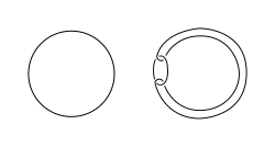
    The unknot (left) and its Bing double (right).

    In knot theory, a field of mathematics, the Bing double of a knot is a link with two components which follow the pattern of the knot and “hook together”. Bing doubles were introduced in Bing (1952) by their namesake, the American mathematician R. H. Bing.[1] The Bing double of a slice knot is a slice link, though it is unknown whether the converse is true.[2] The components of a Bing double bound disjoint Seifert surfaces.[2]

    Bing double
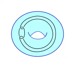
    A solid torus encasing the Bing double of the unknot.

    The Bing double of a knot K is defined by placing the Bing double of the unknot in the solid torus surrounding it, as shown in the figure, and then twisting that solid torus into the shape of K.[2] This definition is similar to that for Whitehead doubles. The Bing double of the unknot is also called the Bing link.[3]

    See also

    References

    Notes

    1. Cimasoni 2006, p. 2395.
    2. 1 2 3 Cimasoni 2006, p. 2397.
    3. Jiang et al. 2002, pp. 189–190.

    Sources

    • Bing, R. H. (1952), “A homeomorphism between the 3-sphere and the sum of two solid horned spheres”, Annals of Mathematics, 56 (2): 354–362.
    • Cimasoni, David (2006), “Slicing Bing doubles”, Algebraic & Geometric Topology, 6: 2395–2415.
    • Jiang, Boju; Lin, Xiao-Song; Wang, Shicheng; Wu, Ying-Qing (2002), “Achirality of knots and links”, Topology and its Applications, 119 (2): 185–208, arXiv:math/9905158, doi:10.1016/S0166-8641(01)00062-1, ISSN 0166-8641.

    Further reading

    • Cochran, Tim; Harvey, Shelly; Leidy, Constance (2008), “Link concordance and generalized doubling operators”, Algebraic & Geometric Topology, 8 (3): 1593–1646, arXiv:0801.3677, doi:10.2140/agt.2008.8.1593.
    • Cha, Jae Choon; Livingston, Charles; Ruberman, Daniel (2008), “Algebraic and Heegaard–Floer invariants of knots with slice Bing doubles”, Mathematical Proceedings of the Cambridge Philosophical Society, 144 (2): 403–410, arXiv:math/0612419, doi:10.1017/S0305004107000795.

    This article is adapted from “Bing double” on Wikipedia, written by its contributors, and used under CC BY-SA 4.0. Text on this page is available under the same licence. Source snapshot: Wikipedia via Kiwix, 2026-07-20.

  • Ply-split braiding

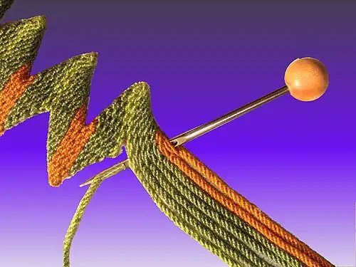
    Ply-split braiding is a technique where one twisted cord (“splitter”) passes through another twisted cord or cords splitting the plies of the latter cords (“splittee” cords). This is unlike weaving or many forms of braiding where cloth is formed by threads interlacing in an over-under sequence. Pattern is formed by cord color, and splitting order.

    A gripfid.
    A cord being pulled through others in ply-split braiding.

    History

    Ply-split braiding is an ancient art that is practiced for making elaborate camel girths and other animal regalia of hand-spun goat hair, wool or sometimes cotton in northwestern India.

    The first written description of the technique appeared in 1976 with Virginia Harvey’s “Split-Ply Twining”.[1] In the introduction, she describes seeing two camel girths at Convergence 1974, and says that Peter Collingwood “suspected the pieces were produced by pulling one yarn through the ply of another”. The ply-split girths examined for this publication were created with only one technique, now known as single course oblique twining (SCOT).

    In 1974 and 1975, two graduate students from UCLA conducted field research in Rajasthan and Gujarat in north-western India. They were introduced to Ishwar Singh, a master girth maker, who spent several weeks with them demonstrating the construction of the girths. Their 1982 publication, “The Ply-Split Camel Girths of West India” [2] was the first to document the entire traditional process, including spinning, plying, cordmaking, and three structures of ply-splitting. These are SCOT, mentioned above, as well as plain oblique twining (POT) and two-layered oblique interlacing (TLOI).

    The designs showed prominence in the market and were even used to decorate camels for wedding processions.[3][4]

    Modern usage

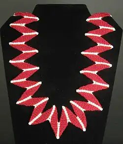
    A Ply-split Braided Necklace
    A braided necklace made from cotton cords by ply-split braiding

    Today, the ply-split braiding technique is used by fiber artists to create handmade decorative items including neckwear, bags, household décor, garments and three-dimensional structures such as baskets and sculptures.[5][6][7][8]

    Contemporary braid makers use a variety of yarns such as cotton, linen, hemp, silk, paper, or rayon. The ply-splitting process requires minimal equipment: A four-hook cord maker[9][10] to make the cords, and a gripfid for splitting the plies of one or more cords and drawing a cord back through the split cords.

    Resources

    The premier reference is Peter Collingwood’s The Techniques of Ply-split Braiding.[11] which presents a comprehensive view of the history and techniques. A more easily accessible history is found in David Fraser’s paper “View From The Shoulders Of Thar Masters: New Space For Ply-Split Braiding”.[12] Other publications include Julie Hedges, Ply-split Braiding, An Introduction[13] and Ply-split Braiding, Further Techniques.[14] Linda Hendrickson’s work includes “Great SCOT! A Beginner’s Guide to Ply-Split Braids in Single-Course Oblique Twining”,[15] “How to Make Ply-Split Baskets”,[16] “How to Make Ply-Split Braids & Bands”,[17] and several instructional videos on YouTube.[18][19][20][21][22][23][24] There have been many publications in weaving journals.[25][26][27][28][29][30][31][32]

    References

    1. “Split-Ply-Twining”, Virginia I. Harvey (1976)”Threads in Action”, Monograph I, HTH Publishers, Santa Ana, California
    2. “Ply-split Camel Girths of West India”, Betsy D. Quick & Judith A. Stein (1982) Pamphlet Series Vol. 1, Number 7, Museum of Cultural History, University of California, Los Angeles.
    3. “Ply-split Braiding: From Camel Girth to Contemporary Craft” http://lsa.uoregon.edu/newsletter04/0411news.html#ply
    4. “Camel regalia”, Julie Hedges (2011), Selvedge issue 38 Jan/Feb 2011.
    5. “The Bowlor Hat.” Collingwood, Peter, Complex Weavers Journal, October 2005, pp. 16–19.
    6. “The Techniques of Ply-split Braiding”, Peter Collingwood (ISBN 0-9625586-9-9)
    7. Beyond Tradition: Contemporary Ply-Split Fiber Sculpture. Portland, OR: Contemporary Crafts Museum & Gallery, 2004. ISBN 0-9728981-1-5 (catalog of a ply-splitting exhibition)
    8. Ply-Splitting in 3 Dimensions: An introduction to making vessels and sculptural forms. Shrewsbury, UK, Author. 2016. ISBN 9780955418723
    9. “Making Cords for Ply-split Braiding. An Overview.” http://www.louisefrench.com/techniques/getting-started/cord-making/overview/overview.html
    10. “Linda Hendrickson Demonstrates Making Cords” https://www.youtube.com/watch?v=JOpomKQe5Oc
    11. Collingwood, Peter. The Techniques of Ply-split Braiding. ISBN 1-85725-133-4.
    12. Fraser, David W. (2010). “View From The Shoulders Of Thar Masters: New Space For Ply-Split Braiding”, Textile Society of America Symposium Proceedings.
    13. Hedges, Julie (2006). Ply-split Braiding, An Introduction. ISBN 978-0-9554187-0-9.
    14. Hedges, Julie (2011). Ply-split Braiding, Further Techniques. ISBN 978-0-9554187-1-6.
    15. Hendrickson, Linda (2000). Great SCOT! A Beginner’s Guide to Ply-Split Braids in Single- Course Oblique Twining.
    16. Hendrickson, Linda (2010). “How to Make Ply-Split Baskets”.
    17. Hendrickson, Linda (2014). “How to Make Ply-Split Braids & Bands”.
    18. “Make the Ply-Split Waves Braid with instructor Linda Hendrickson” https://www.youtube.com/watch?v=vJe2-Pf8fpE
    19. “Ply-Split Braiding: The Waffle Braid” https://www.youtube.com/watch?v=v_QbIBZl8Ss
    20. “Scenes from the DVD ‘Ply-Split Garlic Basket’ with Instructor Linda Hendrickson” https://www.youtube.com/watch?v=xzCHpq8vc6A
    21. “Linda Hendrickson Demonstrates Making Cords” https://www.youtube.com/watch?v=JOpomKQe5Oc
    22. “How to Make a Gripfid for Ply-Splitting” https://www.youtube.com/watch?v=8e9-t9aXa6M
    23. “How to Make Ply-Split Baskets” https://www.youtube.com/watch?v=LDGHQ0awdsM
    24. Hendrickson, Linda. “Tablet Weaving and Ply-Split Braiding“, LindaHendrickson.com.
    25. Collingwood, Peter. “Ply-Split Braiding”, Weaver’s, Issue 29, Fall 1995, pp. 46–51.
    26. Collingwood, Peter. “Ply-Split Braiding Part II”, Weaver’s, Issue 32, Summer 1996, pp. 46–49.
    27. Collingwood, Peter. “Single-Course Oblique Twining”, Weaver’s, Issue 42, Winter 1998, pp. 56–59.
    28. Louise French and Barbara Walker, (Winter, 2008). “Portable, Addictive: Ply-Splitting!“, WeaveZine.
    29. Hendrickson, Linda (September/October 2001). “Star Ornaments in Ply-Split Braiding”, Handwoven, pp. 30–32.
    30. Walker, Barbara (March/April 2011). “Learn Ply-Splitting with Two Summer Trivets”, Handwoven, pp. 40–42.
    31. French, Louise (November/December 2011). “A Tisket, a Tasket, a Ply-Split Basket”, Handwoven, pp. 68–69.
    32. Walker, Barbara J. (2012) Ply-Splitting from Drawdowns: Interpreting Weave Structures in Ply-Split Braiding. ISBN 978-0-9856293-0-4

    This article is adapted from “Ply-split braiding” on Wikipedia, written by its contributors, and used under CC BY-SA 4.0. Text on this page is available under the same licence. Source snapshot: Wikipedia via Kiwix, 2026-07-20.

  • Planar algebra

    In mathematics, planar algebras first appeared in the work of Vaughan Jones on the standard invariant of a II1 subfactor.[1] They also provide an appropriate algebraic framework for many knot invariants (in particular the Jones polynomial), and have been used in describing the properties of Khovanov homology with respect to tangle composition.[2][3] Any subfactor planar algebra provides a family of unitary representations of Thompson groups.[4]
    Any finite group (and quantum generalization) can be encoded as a planar algebra.[1]

    Definition

    The idea of the planar algebra is to be a diagrammatic axiomatization of the standard invariant.[1][5][6]

    Planar tangle

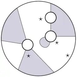
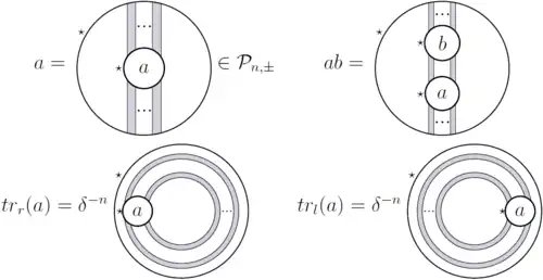
    A (shaded) planar tangle is the data of finitely many input disks, one output disk, non-intersecting strings giving an even number, say 2 n {\displaystyle 2n} {\displaystyle 2n}, intervals per disk and one {\displaystyle \star } {\displaystyle \star }-marked interval per disk.

    Planar algebra

    Here, the mark is shown as a {\displaystyle \star } {\displaystyle \star }-shape. On each input disk it is placed between two adjacent outgoing strings, and on the output disk it is placed between two adjacent incoming strings. A planar tangle is defined up to isotopy.

    Composition

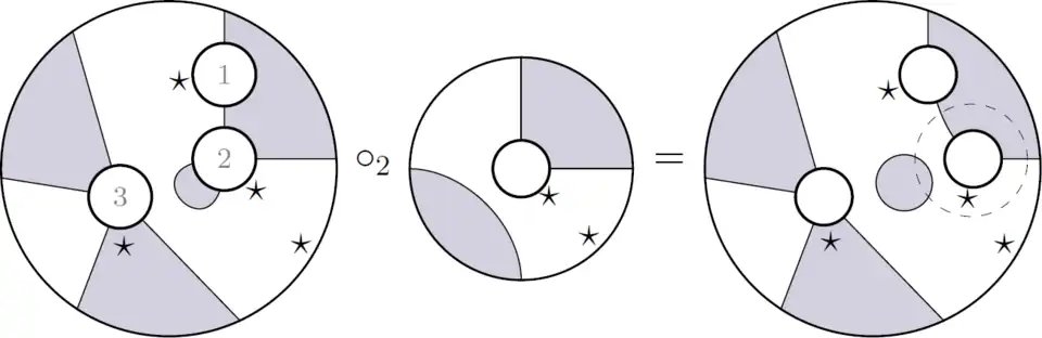
    To compose two planar tangles, put the output disk of one into an input of the other, having as many intervals, same shading of marked intervals and such that the {\displaystyle \star } {\displaystyle \star }-marked intervals coincide. Finally we remove the coinciding circles. Note that two planar tangles can have zero, one or several possible compositions.

    Planar algebra

    Planar operad

    The planar operad is the set of all the planar tangles (up to isomorphism) with such compositions.

    Planar algebra

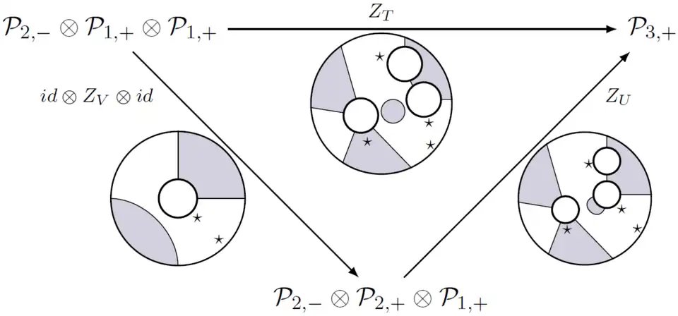
    A planar algebra is a representation of the planar operad; more precisely, it is a family of vector spaces ( P n , ± ) n N {\displaystyle ({\mathcal {P}}_{n,\pm })_{n\in \mathbb {N} }} {\displaystyle ({\mathcal {P}}_{n,\pm })_{n\in \mathbb {N} }}, called n {\displaystyle n} {\displaystyle n}-box spaces, on which acts the planar operad, i.e. for any tangle T {\displaystyle T} {\displaystyle T} (with one output disk and r {\displaystyle r} {\displaystyle r} input disks with 2 n 0 {\displaystyle 2n_{0}} {\displaystyle 2n_{0}} and 2 n 1 , , 2 n r {\displaystyle 2n_{1},\dots ,2n_{r}} {\displaystyle 2n_{1},\dots ,2n_{r}} intervals respectively) there is a multilinear map

    Z T : P n 1 , ϵ 1 P n r , ϵ r P n 0 , ϵ 0 {\displaystyle Z_{T}:{\mathcal {P}}_{n_{1},\epsilon _{1}}\otimes \cdots \otimes {\mathcal {P}}_{n_{r},\epsilon _{r}}\to {\mathcal {P}}_{n_{0},\epsilon _{0}}} {\displaystyle Z_{T}:{\mathcal {P}}_{n_{1},\epsilon _{1}}\otimes \cdots \otimes {\mathcal {P}}_{n_{r},\epsilon _{r}}\to {\mathcal {P}}_{n_{0},\epsilon _{0}}}

    with ϵ i { + , } {\displaystyle \epsilon _{i}\in \{+,-\}} {\displaystyle \epsilon _{i}\in \{+,-\}} according to the shading of the {\displaystyle \star } {\displaystyle \star }-marked intervals, and these maps (also called partition functions) respect the composition of tangle in such a way that all the diagrams as below commute.

    Planar algebra

    Examples

    Planar tangles

    The family of vector spaces ( T n , ± ) n N {\displaystyle ({\mathcal {T}}_{n,\pm })_{n\in \mathbb {N} }} {\displaystyle ({\mathcal {T}}_{n,\pm })_{n\in \mathbb {N} }} generated by the planar tangles having 2 n {\displaystyle 2n} {\displaystyle 2n} intervals on their output disk and a white (or black) {\displaystyle \star } {\displaystyle \star }-marked interval, admits a planar algebra structure.

    Temperley–Lieb

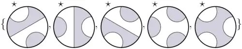
    The Temperley-Lieb planar algebra T L ( δ ) {\displaystyle {\mathcal {TL}}(\delta )} {\displaystyle {\mathcal {TL}}(\delta )} is generated by the planar tangles without input disk; its 3 {\displaystyle 3} {\displaystyle 3}-box space T L 3 , + ( δ ) {\displaystyle {\mathcal {TL}}_{3,+}(\delta )} {\displaystyle {\mathcal {TL}}_{3,+}(\delta )} is generated by

    Planar algebra

    Moreover, a closed string is replaced by a multiplication by δ {\displaystyle \delta } {\displaystyle \delta }.

    Planar algebra

    Note that the dimension of T L n , ± ( δ ) {\displaystyle {\mathcal {TL}}_{n,\pm }(\delta )} {\displaystyle {\mathcal {TL}}_{n,\pm }(\delta )} is the Catalan number 1 n + 1 ( 2 n n ) {\displaystyle {\frac {1}{n+1}}{\binom {2n}{n}}} {\displaystyle {\frac {1}{n+1}}{\binom {2n}{n}}}.
    This planar algebra encodes the notion of Temperley–Lieb algebra.

    Hopf algebra

    A semisimple and cosemisimple Hopf algebra over an algebraically closed field is encoded in a planar algebra defined by generators and relations, and “corresponds” (up to isomorphism) to a connected, irreducible, spherical, non degenerate planar algebra with non zero modulus δ {\displaystyle \delta } {\displaystyle \delta } and of depth two.[7]

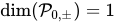
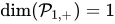
    Note that connected means dim ( P 0 , ± ) = 1 {\displaystyle \dim({\mathcal {P}}_{0,\pm })=1} {\displaystyle \dim({\mathcal {P}}_{0,\pm })=1} (as for evaluable below), irreducible means dim ( P 1 , + ) = 1 {\displaystyle \dim({\mathcal {P}}_{1,+})=1} {\displaystyle \dim({\mathcal {P}}_{1,+})=1}, spherical is defined below, and non-degenerate means that the traces (defined below) are non-degenerate.

    Subfactor planar algebra

    Definition

    A subfactor planar algebra is a planar {\displaystyle \star } {\displaystyle \star }-algebra ( P n , ± ) n N {\displaystyle ({\mathcal {P}}_{n,\pm })_{n\in \mathbb {N} }} {\displaystyle ({\mathcal {P}}_{n,\pm })_{n\in \mathbb {N} }} which is:

    (1) Finite-dimensional: dim ( P n , ± ) < {\displaystyle \dim({\mathcal {P}}_{n,\pm })<\infty } {\displaystyle \dim({\mathcal {P}}_{n,\pm })<\infty }
    (2) Evaluable: P 0 , ± = C {\displaystyle {\mathcal {P}}_{0,\pm }=\mathbb {C} } {\displaystyle {\mathcal {P}}_{0,\pm }=\mathbb {C} }
    (3) Spherical: t r := t r r = t r l {\displaystyle tr:=tr_{r}=tr_{l}} {\displaystyle tr:=tr_{r}=tr_{l}}
    (4) Positive: a | b = t r ( b a ) {\displaystyle \langle a\vert b\rangle =tr(b^{\star }a)} {\displaystyle \langle a\vert b\rangle =tr(b^{\star }a)} defines an inner product.

    Note that by (2) and (3), any closed string (shaded or not) counts for the same constant δ {\displaystyle \delta } {\displaystyle \delta }.

    Planar algebra

    The tangle action deals with the adjoint by:

    Z T ( a 1 a 2 a r ) = Z T ( a 1 a 2 a r ) {\displaystyle Z_{T}(a_{1}\otimes a_{2}\otimes \cdots \otimes a_{r})^{\star }=Z_{T^{\star }}(a_{1}^{\star }\otimes a_{2}^{\star }\otimes \cdots \otimes a_{r}^{\star })} {\displaystyle Z_{T}(a_{1}\otimes a_{2}\otimes \cdots \otimes a_{r})^{\star }=Z_{T^{\star }}(a_{1}^{\star }\otimes a_{2}^{\star }\otimes \cdots \otimes a_{r}^{\star })}

    with T {\displaystyle T^{\star }} {\displaystyle T^{\star }} the mirror image of T {\displaystyle T} {\displaystyle T} and a i {\displaystyle a_{i}^{\star }} {\displaystyle a_{i}^{\star }} the adjoint of a i {\displaystyle a_{i}} {\displaystyle a_{i}} in P n i , ϵ i {\displaystyle {\mathcal {P}}_{n_{i},\epsilon _{i}}} {\displaystyle {\mathcal {P}}_{n_{i},\epsilon _{i}}}.

    Examples and results

    No-ghost theorem: The planar algebra T L ( δ ) {\displaystyle {\mathcal {TL}}(\delta )} {\displaystyle {\mathcal {TL}}(\delta )} has no ghost (i.e. element a {\displaystyle a} {\displaystyle a} with a | a < 0 {\displaystyle \langle a\vert a\rangle <0} {\displaystyle \langle a\vert a\rangle <0}) if and only if

    δ { 2 cos ( π / n ) | n = 3 , 4 , 5 , . . . } [ 2 , + ] {\displaystyle \delta \in \{2\cos(\pi /n)|n=3,4,5,…\}\cup [2,+\infty ]} {\displaystyle \delta \in \{2\cos(\pi /n)|n=3,4,5,...\}\cup [2,+\infty ]}

    For δ {\displaystyle \delta } {\displaystyle \delta } as above, let I {\displaystyle {\mathcal {I}}} {\displaystyle {\mathcal {I}}} be the null ideal (generated by elements a {\displaystyle a} {\displaystyle a} with a | a = 0 {\displaystyle \langle a\vert a\rangle =0} {\displaystyle \langle a\vert a\rangle =0}). Then the quotient T L ( δ ) / I {\displaystyle {\mathcal {TL}}(\delta )/{\mathcal {I}}} {\displaystyle {\mathcal {TL}}(\delta )/{\mathcal {I}}} is a subfactor planar algebra, called the Temperley–Lieb-Jones subfactor planar algebra T L J ( δ ) {\displaystyle {\mathcal {TLJ}}(\delta )} {\displaystyle {\mathcal {TLJ}}(\delta )}. Any subfactor planar algebra with constant δ {\displaystyle \delta } {\displaystyle \delta } admits T L J ( δ ) {\displaystyle {\mathcal {TLJ}}(\delta )} {\displaystyle {\mathcal {TLJ}}(\delta )} as planar subalgebra.

    A planar algebra ( P n , ± ) {\displaystyle ({\mathcal {P}}_{n,\pm })} {\displaystyle ({\mathcal {P}}_{n,\pm })} is a subfactor planar algebra if and only if it is the standard invariant of an extremal subfactor N M {\displaystyle N\subseteq M} {\displaystyle N\subseteq M} of index [ M : N ] = δ 2 {\displaystyle [M:N]=\delta ^{2}} {\displaystyle [M:N]=\delta ^{2}}, with P n , + = N M n 1 {\displaystyle {\mathcal {P}}_{n,+}=N’\cap M_{n-1}} {\displaystyle {\mathcal {P}}_{n,+}=N'\cap M_{n-1}} and P n , = M M n {\displaystyle {\mathcal {P}}_{n,-}=M’\cap M_{n}} {\displaystyle {\mathcal {P}}_{n,-}=M'\cap M_{n}}.[8][9][10]
    A finite depth or irreducible subfactor is extremal ( t r N = t r M {\displaystyle tr_{N’}=tr_{M}} {\displaystyle tr_{N'}=tr_{M}} on N M {\displaystyle N’\cap M} {\displaystyle N'\cap M}).

    There is a subfactor planar algebra encoding any finite group (and more generally, any finite dimensional Hopf C {\displaystyle {\rm {C}}^{\star }} {\displaystyle {\rm {C}}^{\star }}-algebra, called Kac algebra), defined by generators and relations. A (finite dimensional) Kac algebra “corresponds” (up to isomorphism) to an irreducible subfactor planar algebra of depth two.[11][12]

    The subfactor planar algebra associated to an inclusion of finite groups,[13]
    does not always remember the (core-free) inclusion.[14][15]

    A Bisch-Jones subfactor planar algebra B J ( δ 1 , δ 2 ) {\displaystyle {\mathcal {BJ}}(\delta _{1},\delta _{2})} {\displaystyle {\mathcal {BJ}}(\delta _{1},\delta _{2})} (sometimes called Fuss-Catalan) is defined as for T L J ( δ ) {\displaystyle {\mathcal {TLJ}}(\delta )} {\displaystyle {\mathcal {TLJ}}(\delta )} but by allowing two colors of string with their own constant δ 1 {\displaystyle \delta _{1}} {\displaystyle \delta _{1}} and δ 2 {\displaystyle \delta _{2}} {\displaystyle \delta _{2}}, with δ i {\displaystyle \delta _{i}} {\displaystyle \delta _{i}} as above. It is a planar subalgebra of any subfactor planar algebra with an intermediate such that [ K : N ] = δ 1 2 {\displaystyle [K:N]=\delta _{1}^{2}} {\displaystyle [K:N]=\delta _{1}^{2}} and [ M : K ] = δ 2 2 {\displaystyle [M:K]=\delta _{2}^{2}} {\displaystyle [M:K]=\delta _{2}^{2}}.[16][17]

    The first finite depth subfactor planar algebra of index δ 2 > 4 {\displaystyle \delta ^{2}>4} {\displaystyle \delta ^{2}>4} is called the Haagerup subfactor planar algebra.[18] It has index ( 5 + 13 ) / 2 4.303 {\displaystyle (5+{\sqrt {13}})/2\sim 4.303} {\displaystyle (5+{\sqrt {13}})/2\sim 4.303}.

    The subfactor planar algebras are completely classified for index at most 5 {\displaystyle 5} {\displaystyle 5}[19]
    and a bit beyond.[20]
    This classification was initiated by Uffe Haagerup.[21]
    It uses (among other things) a listing of possible principal graphs, together with the embedding theorem[22]
    and the jellyfish algorithm.[23]

    A subfactor planar algebra remembers the subfactor (i.e. its standard invariant is complete) if it is amenable.[24]
    A finite depth hyperfinite subfactor is amenable.

    About the non-amenable case: there are unclassifiably many irreducible hyperfinite subfactors of index 6 that all have the same standard invariant.[25]

    Fourier transform and biprojections

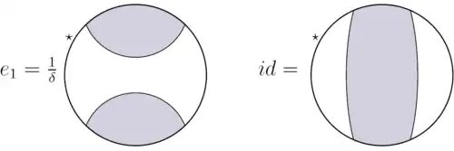
    Let N M {\displaystyle N\subset M} {\displaystyle N\subset M} be a finite index subfactor, and P {\displaystyle {\mathcal {P}}} {\displaystyle {\mathcal {P}}} the corresponding subfactor planar algebra. Assume that P {\displaystyle {\mathcal {P}}} {\displaystyle {\mathcal {P}}} is irreducible (i.e. P 1 , + = N M 1 = C {\displaystyle {\mathcal {P}}_{1,+}=N’\cap M_{1}=\mathbb {C} } {\displaystyle {\mathcal {P}}_{1,+}=N'\cap M_{1}=\mathbb {C} }). Let N K M {\displaystyle N\subset K\subset M} {\displaystyle N\subset K\subset M} be an intermediate subfactor. Let the Jones projection e K M : L 2 ( M ) L 2 ( K ) {\displaystyle e_{K}^{M}:L^{2}(M)\to L^{2}(K)} {\displaystyle e_{K}^{M}:L^{2}(M)\to L^{2}(K)}. Note that e K M P 2 , + {\displaystyle e_{K}^{M}\in {\mathcal {P}}_{2,+}} {\displaystyle e_{K}^{M}\in {\mathcal {P}}_{2,+}}. Let i d := e M M {\displaystyle id:=e_{M}^{M}} {\displaystyle id:=e_{M}^{M}} and e 1 := e N M {\displaystyle e_{1}:=e_{N}^{M}} {\displaystyle e_{1}:=e_{N}^{M}}.

    Planar algebra

    Note that t r ( e 1 ) = δ 2 = [ M : N ] 1 {\displaystyle tr(e_{1})=\delta ^{-2}=[M:N]^{-1}} {\displaystyle tr(e_{1})=\delta ^{-2}=[M:N]^{-1}} and t r ( i d ) = 1 {\displaystyle tr(id)=1} {\displaystyle tr(id)=1}.

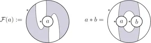
    Let the bijective linear map F : P 2 , ± P 2 , {\displaystyle {\mathcal {F}}:{\mathcal {P}}_{2,\pm }\to {\mathcal {P}}_{2,\mp }} {\displaystyle {\mathcal {F}}:{\mathcal {P}}_{2,\pm }\to {\mathcal {P}}_{2,\mp }} be the Fourier transform, also called 1 {\displaystyle 1} {\displaystyle 1}-click (of the outer star) or 90 {\displaystyle 90^{\circ }} {\displaystyle 90^{\circ }} rotation; and let a b {\displaystyle a*b} {\displaystyle a*b} be the coproduct of a {\displaystyle a} {\displaystyle a} and b {\displaystyle b} {\displaystyle b}.

    Planar algebra

    Note that the word coproduct is a diminutive of convolution product. It is a binary operation.

    The coproduct satisfies the equality a b = F ( F 1 ( a ) F 1 ( b ) ) . {\displaystyle a*b={\mathcal {F}}({\mathcal {F}}^{-1}(a){\mathcal {F}}^{-1}(b)).} {\displaystyle a*b={\mathcal {F}}({\mathcal {F}}^{-1}(a){\mathcal {F}}^{-1}(b)).}

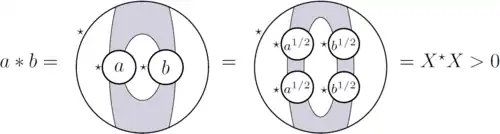
    For any positive operators a , b {\displaystyle a,b} {\displaystyle a,b}, the coproduct a b {\displaystyle a*b} {\displaystyle a*b} is also positive; this can be seen diagrammatically:[26]

    Planar algebra

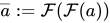
    Let a ¯ := F ( F ( a ) ) {\displaystyle {\overline {a}}:={\mathcal {F}}({\mathcal {F}}(a))} {\displaystyle {\overline {a}}:={\mathcal {F}}({\mathcal {F}}(a))} be the contragredient a {\displaystyle a} {\displaystyle a} (also called 180 {\displaystyle 180^{\circ }} {\displaystyle 180^{\circ }} rotation). The map F 4 {\displaystyle {\mathcal {F}}^{4}} {\displaystyle {\mathcal {F}}^{4}} corresponds to four 1 {\displaystyle 1} {\displaystyle 1}-clicks of the outer star, so it’s the identity map, and then a ¯ ¯ = a {\displaystyle {\overline {\overline {a}}}=a} {\displaystyle {\overline {\overline {a}}}=a}.

    In the Kac algebra case, the contragredient is exactly the antipode,[12] which, for a finite group, correspond to the inverse.

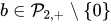
    A biprojection is a projection b P 2 , + { 0 } {\displaystyle b\in {\mathcal {P}}_{2,+}\setminus \{0\}} {\displaystyle b\in {\mathcal {P}}_{2,+}\setminus \{0\}} with F ( b ) {\displaystyle {\mathcal {F}}(b)} {\displaystyle {\mathcal {F}}(b)} a multiple of a projection.
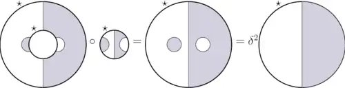
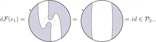
    Note that e 1 = e N M {\displaystyle e_{1}=e_{N}^{M}} {\displaystyle e_{1}=e_{N}^{M}} and i d = e M M {\displaystyle id=e_{M}^{M}} {\displaystyle id=e_{M}^{M}} are biprojections; this can be seen as follows:

    Planar algebra

    A projection b {\displaystyle b} {\displaystyle b} is a biprojection iff it is the Jones projection e K M {\displaystyle e_{K}^{M}} {\displaystyle e_{K}^{M}} of an intermediate subfactor N K M {\displaystyle N\subset K\subset M} {\displaystyle N\subset K\subset M},[27] iff e 1 b = b ¯ = λ b b ,  with  λ 1 = δ t r ( b ) {\displaystyle e_{1}\leq b={\overline {b}}=\lambda b*b,{\text{ with }}\lambda ^{-1}=\delta tr(b)} {\displaystyle e_{1}\leq b={\overline {b}}=\lambda b*b,{\text{ with }}\lambda ^{-1}=\delta tr(b)}.[28][26]

    Galois correspondence:[29] in the Kac algebra case, the biprojections are 1-1 with the left coideal subalgebras, which, for a finite group, correspond to the subgroups.

    For any irreducible subfactor planar algebra, the set of biprojections is a finite lattice,[30] of the form [ e 1 , i d ] {\displaystyle [e_{1},id]} {\displaystyle [e_{1},id]}, as for an interval of finite groups [ H , G ] {\displaystyle [H,G]} {\displaystyle [H,G]}.

    Using the biprojections, we can make the intermediate subfactor planar algebras.[31][32]

    The uncertainty principle extends to any irreducible subfactor planar algebra P {\displaystyle {\mathcal {P}}} {\displaystyle {\mathcal {P}}}:

    Let S ( x ) = T r ( R ( x ) ) {\displaystyle {\mathcal {S}}(x)=Tr(R(x))} {\displaystyle {\mathcal {S}}(x)=Tr(R(x))} with R ( x ) {\displaystyle R(x)} {\displaystyle R(x)} the range projection of x {\displaystyle x} {\displaystyle x} and T r {\displaystyle Tr} {\displaystyle Tr} the unnormalized trace (i.e. T r = δ n t r {\displaystyle Tr=\delta ^{n}tr} {\displaystyle Tr=\delta ^{n}tr} on P n , ± {\displaystyle {\mathcal {P}}_{n,\pm }} {\displaystyle {\mathcal {P}}_{n,\pm }}).

    Noncommutative uncertainty principle:[33] Let x P 2 , ± {\displaystyle x\in {\mathcal {P}}_{2,\pm }} {\displaystyle x\in {\mathcal {P}}_{2,\pm }}, nonzero. Then

    S ( x ) S ( F ( x ) ) δ 2 {\displaystyle {\mathcal {S}}(x){\mathcal {S}}({\mathcal {F}}(x))\geq \delta ^{2}} {\displaystyle {\mathcal {S}}(x){\mathcal {S}}({\mathcal {F}}(x))\geq \delta ^{2}}

    Assuming x {\displaystyle x} {\displaystyle x} and F ( x ) {\displaystyle {\mathcal {F}}(x)} {\displaystyle {\mathcal {F}}(x)} positive, the equality holds if and only if x {\displaystyle x} {\displaystyle x} is a biprojection. More generally, the equality holds if and only if x {\displaystyle x} {\displaystyle x} is the bi-shift of a biprojection.

    References

    1. 1 2 3
      Vaughan F. R. Jones (1999), “Planar algebras, I”, arXiv:math/9909027
    2. Bar-Natan, Dror (2004), “Dror Bar-Natan: Publications: Cobordisms”, Math.toronto.edu, pp. 1443–1499, arXiv:math/0410495, doi:10.2140/gt.2005.9.1443, retrieved 2016-11-20
    3. Bar-Natan, Dror (2005), “Khovanov’s homology for tangles and cobordisms”, Geometry & Topology, 9 (3): 1443–1499, arXiv:math/0410495, doi:10.2140/gt.2005.9.1443, S2CID 1247623

    4. Vaughan F. R. Jones (2017), “Some unitary representations of Thompson’s groups F and T”, J. Comb. Algebra, 1 (1): 1–44, arXiv:1412.7740, doi:10.4171/JCA/1-1-1, MR 3589908, S2CID 119631229

    5. Vijay Kodiyalam; V.S. Sunder (2004), “On Jones’ planar algebras”, J. Knot Theory Ramifications, 13 (2): 219–247, doi:10.1142/S021821650400310X, MR 2047470

    6. “Vijay Kodiyalam – Planar algebras – IMSc 2015”, youtube.com, 2015-11-14

    7. Vijay Kodiyalam; V.S. Sunder (2006), “The planar algebra of a semisimple and cosemisimple Hopf algebra”, Proc. Indian Acad. Sci. Math. Sci., 116 (4): 1–16, arXiv:math/0506153, Bibcode:2005math……6153K

    8. Sorin Popa (1995), “An axiomatization of the lattice of higher relative commutants of a subfactor”, Inventiones Mathematicae, 120 (3): 427–445, Bibcode:1995InMat.120..427P, doi:10.1007/BF01241137, MR 1334479, S2CID 1740471

    9. Alice Guionnet; Vaughan F. R. Jones; Dimitri Shlyakhtenko (2010), “Random matrices, free probability, planar algebras and subfactors”, Clay Math. Proc., {11}: 201–239, MR 2732052

    10. Vijay Kodiyalam; V.S. Sunder (2009), “From subfactor planar algebras to subfactors”, Internat. J. Math., 20 (10): 1207–1231, arXiv:0807.3704, doi:10.1142/S0129167X0900573X, MR 2574313, S2CID 115161031

    11. Paramita Das; Vijay Kodiyalam (2005), “Planar algebras and the Ocneanu-Szymanski theorem”, Proc. Amer. Math. Soc., 133 (9): 2751–2759, doi:10.1090/S0002-9939-05-07789-0, ISSN 0002-9939, MR 2146224
    12. 1 2
      Vijay Kodiyalam; Zeph Landau; V.S. Sunder (2003), “The planar algebra associated to a Kac algebra”, Proc. Indian Acad. Sci. Math. Sci., 113 (1): 15–51, doi:10.1007/BF02829677, ISSN 0253-4142, MR 1971553, S2CID 56571515

    13. Ved Prakash Gupta (2008), “Planar algebra of the subgroup-subfactor”, Proceedings Mathematical Sciences, 118 (4): 583–612, arXiv:0806.1791, Bibcode:2008arXiv0806.1791G, doi:10.1007/s12044-008-0046-0, S2CID 5589336

    14. Vijay Kodiyalam; V.S. Sunder (2000), “The subgroup-subfactor”, Math. Scand., 86 (1): 45–74, doi:10.7146/math.scand.a-14281, ISSN 0025-5521, MR 1738515

    15. Masaki Izumi (2002), “Characterization of isomorphic group-subgroup subfactors”, Int. Math. Res. Not., 2002 (34): 1791–1803, doi:10.1155/S107379280220402X, ISSN 1073-7928, MR 1920326{{citation}}: CS1 maint: unflagged free DOI (link)
    16. Dietmar Bisch; Vaughan Jones (1997), “Algebras associated to intermediate subfactors”, Inventiones Mathematicae, 128 (1): 89–157, Bibcode:1997InMat.128…89J, doi:10.1007/s002220050137, S2CID 119372640

    17. Pinhas Grossman; Vaughan Jones (2007), “Intermediate subfactors with no extra structure”, J. Amer. Math. Soc., 20 (1): 219–265, Bibcode:2007JAMS…20..219G, doi:10.1090/S0894-0347-06-00531-5, MR 2257402

    18. Emily Peters (2010), “A planar algebra construction of the Haagerup subfactor”, Internat. J. Math., 21 (8): 987–1045, arXiv:0902.1294, doi:10.1142/S0129167X10006380, MR 2679382, S2CID 951475

    19. Vaughan F. R. Jones; Scott Morrison; Noah Snyder (2014), “The classification of subfactors of index at most 5 {\displaystyle 5} {\displaystyle 5}“, Bull. Amer. Math. Soc. (N.S.), 51 (2): 277–327, arXiv:1304.6141, doi:10.2140/gt.2005.9.1443, MR 3166042, S2CID 29962597

    20. Narjess Afzaly; Scott Morrison; David Penneys (2015), The classification of subfactors with index at most 5 + 1 / 4 {\displaystyle 5+1/4} {\displaystyle 5+1/4}, pp. 70pp, arXiv:1509.00038, Bibcode:2015arXiv150900038A

    21. Uffe Haagerup (1994), “Principal graphs of subfactors in the index range 4 < [ M : N ] < 3 + 2 {\displaystyle 4<[M:N]<3+{\sqrt {2}}} {\displaystyle 4<[M:N]<3+{\sqrt {2}}}“, Subfactors (Kyuzeso, 1993): 1–38, MR 1317352

    22. Vaughan Jones; David Penneys (2011), “The embedding theorem for finite depth subfactor planar algebras.”, Quantum Topol., 2 (3): 301–337, arXiv:1007.3173, doi:10.4171/QT/23, MR 2812459, S2CID 59578009

    23. Stephen Bigelow; David Penneys (2014), “Principal graph stability and the jellyfish algorithm.”, Math. Ann., 358 (1–2): 1–24, arXiv:1208.1564, doi:10.1007/s00208-013-0941-2, MR 3157990, S2CID 3549669

    24. Popa, Sorin (1994), “Classification of amenable subfactors of type II”, Acta Mathematica, 172 (2): 163–255, doi:10.1007/BF02392646, MR 1278111

    25. Arnaud Brothier; Stefaan Vaes (2015), “Families of hyperfinite subfactors with the same standard invariant and prescribed fundamental group.”, J. Noncommut. Geom., 9 (3): 775–796, arXiv:1309.5354, doi:10.4171/JNCG/207, MR 3420531, S2CID 117853753
    26. 1 2
      Zhengwei Liu (2016), “Exchange relation planar algebras of small rank”, Trans. Amer. Math. Soc., 368 (12): 8303–8348, arXiv:1308.5656, doi:10.1090/tran/6582, ISSN 0002-9947, MR 3551573, S2CID 117030298

    27. Dietmar Bisch (1994), “A note on intermediate subfactors”, Pacific J. Math., 163 (2): 201–216, doi:10.2140/pjm.1994.163.201, ISSN 0030-8730, MR 1262294

    28. Zeph A. Landau (2002), “Exchange relation planar algebras”, Geom. Dedicata, 95: 183–214, doi:10.1023/A:1021296230310, ISSN 0046-5755, MR 1950890, S2CID 119036175

    29. Masaki Izumi; Roberto Longo; Sorin Popa (1998), “A Galois correspondence for compact groups of automorphisms of von Neumann algebras with a generalization to Kac algebras”, J. Funct. Anal., 155 (1): 25–63, arXiv:funct-an/9604004, doi:10.1006/jfan.1997.3228, ISSN 0022-1236, MR 1622812, S2CID 12990106

    30. Yasuo Watatani (1996), “Lattices of intermediate subfactors”, J. Funct. Anal., 140 (2): 312–334, doi:10.1006/jfan.1996.0110, hdl:2115/68899, ISSN 0022-1236, MR 1409040

    31. Zeph A. Landau (1998), “Intermediate subfactors”, Thesis – University of California at Berkeley: 132pp

    32. Keshab Chandra Bakshi (2016), “Intermediate planar algebra revisited”, International Journal of Mathematics, 29 (12): 31pp, arXiv:1611.05811, Bibcode:2016arXiv161105811B, doi:10.1142/S0129167X18500775, S2CID 119305436

    33. Chunlan Jiang; Zhengwei Liu; Jinsong Wu (2016), “Noncommutative uncertainty principles”, J. Funct. Anal., 270 (1): 264–311, arXiv:1408.1165, doi:10.1016/j.jfa.2015.08.007, S2CID 16295570

    This article is adapted from “Planar algebra” on Wikipedia, written by its contributors, and used under CC BY-SA 4.0. Text on this page is available under the same licence. Source snapshot: Wikipedia via Kiwix, 2026-07-20.

  • Bimini twist

    Bimini twist
    Bimini twist

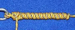
    The Bimini twist [1] is a fishing knot used for offshore trolling and sportsfishing and the creation of double-line leaders.

    Description

    A Bimini twist creates a loop at the end of the line in which it is tied. The loop is secured at the top with a long barrel of coiled line created by the tying process. A Bimini twist loop is stronger than the line itself. It is one of the rare knots that does not weaken the line in which it is tied. It is a simple method of doubling your fishing line in order to prevent chafing or to create the necessary loop in order to attach a wind-on leader without using strength in the mainline. For use in fishing applications, the old standby is 20-30 initial twists in nylon monofilament and 60 or more initial-twists in Spectra-type braided line.

    An article in Sportfishing Magazine in February 2007 made the claim that fewer twists created greater strength. However, the holding mechanism in a Bimini Twist is the friction created by the twists. It was quickly and has since been often demonstrated that the 12-twist knot (proposed in the article) in Spectra-braid slipped before breaking. It is not known what testing errors led to the erroneous conclusion that fewer twists made a stronger knot.

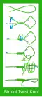
    • How to tie a Bimini twist
      How to tie a Bimini twist
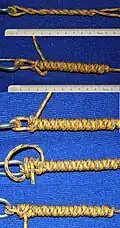
    • How to tie a Bimini twist
      How to tie a Bimini twist
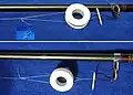
    • Tie with help
      Tie with help

    References

    1. The complete guide to knots and knot tying — Geoffrey Budworth — p.201 — ISBN 0-7548-0422-4

    External links


    This article is adapted from “Bimini twist” on Wikipedia, written by its contributors, and used under CC BY-SA 4.0. Text on this page is available under the same licence. Source snapshot: Wikipedia via Kiwix, 2026-07-20.