In mathematics, biquandles and biracks are sets with binary operations that generalize quandles and racks. In the theory of virtual knots, biquandles are analagous to quandles in the theory of classical knots. Biracks and racks have the same relation, while a biquandle is a birack which satisfies some additional conditions.
Definitions
A birack is a set  , two right-invertible operations
 and a bijection
  such that for all
  ,
,
1. 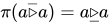 and
and 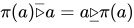 .
.
2. The map  defined by
  is invertible.
3. The exchange laws


 .
.
If  is the identity map,
  is called a biquandle.[1]
Biracks and biquandles were first introduced by Roger Fenn, Mercedes Jordan-Santana and Louis Kauffman in 2004.[2]
Note that the three conditions above correspond directly to the three Reidemeister moves in knot therory, showing the close connections between knots and biracks.[3]
Examples
Let be a set with two bijection  that commute. Then the constant action birack is defined by
  and
and  and
and  .
.
Any rack  is a birack with
  and
and  for all
  . Note that if we insert these operations into the conditions in the definition above, we regain the exact definition of a rack.
Let  be a commutative ring with identity and an
 ![{\displaystyle R[s^{\pm 1},t^{\pm 1}]}](/wp-content/uploads/wiki-images/091acb9bb45467868e570a2b07482c12c336136f-d4d4627c.svg) -module. Then the Alexander biquandle is defined as
-module. Then the Alexander biquandle is defined as  and
and  . For
. For  this is a quandle.
Linear biquandles
Application to virtual links and braids
Birack homology
References
- ↑ Elhamdadi, Mohamed; Nelson, Sam (2015). Quandles: an introduction to the algebra of knots. Student mathematical library. Providence: American mathematical society. ISBN 978-1-4704-2213-4.
- ↑ Fenn, Roger; Jordan-Santana, Mercedes; Kauffman, Louis (2004-11-28). “Biquandles and virtual links”. Topology and its Applications. 145 (1): 157–175. doi:10.1016/j.topol.2004.06.008. ISSN 0166-8641.
- ↑ Pflume, Runa (2024-04-10). Generalizations of Quandles to Multi-Linkoids (masterThesis thesis). doi:10.53846/goediss-10442.
Further reading
- Fenn, Roger; Jordan-Santana, Mercedes; Kauffman, Louis (2004). “Biquandles and Virtual Links”. Topology and its Applications. 145 (1–3): 157–175. doi:10.1016/j.topol.2004.06.008.
- Fenn, Roger; Rourke, Colin; Sanderson, Brian (1993). “An Introduction to Species and the Rack Space”. Topics in Knot Theory. NATO ASI Series. Vol. 399. Springer. pp. 33–55. doi:10.1007/978-94-011-1695-4_4.
- Kauffman, Louis H. (1999). “Virtual Knot Theory”. European Journal of Combinatorics. 20 (7): 663–690. doi:10.1006/eujc.1999.0314.
This article is adapted from “Biracks and biquandles” on Wikipedia, written by its contributors, and used under CC BY-SA 4.0. Text on this page is available under the same licence. Source snapshot: Wikipedia via Kiwix, 2026-07-20.