Blog

  • Ashley’s stopper knot

    Ashley’s stopper knot
    Ashley's stopper knot
    Names Ashley’s stopper knot, Ashley stopper knot, Oysterman’s stopper
    Category Stopper
    Origin Clifford Ashley, c. 1910
    ABoK #526
    A/B notation 820
    Ashley's stopper knot
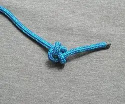
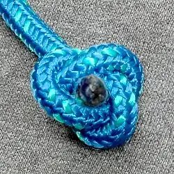
    The load-bearing face of an Ashley’s stopper knot. This particular example was tied in an unusual manner, with what would normally be considered the “standing part” very short, to fully expose the knot’s Trefoil-like face.

    Ashley’s stopper knot, also known as the oysterman’s stopper, is a knot developed by Clifford W. Ashley around 1910. It makes a well-balanced trefoil-faced stopper at the end of the rope, giving greater resistance to pulling through an opening than other common stoppers. Essentially, the knot is a common overhand noose, but with the end of the rope passing through the noose eye, which closes upon it. It may be multiplied to form a larger knot with more than three bights appearing around the knot. It is the result of implementing a double wall knot in one strand.

    Ashley developed this knot in trying to duplicate a knot he saw on a boat in a local oyster fishing fleet. When he had a chance to observe the knot up close at a later time he realized it was just a badly water-swollen figure eight stopper knot.[1]

    The oysterman’s stopper…It is a larger knot than the figure-eight, which has but one part around the stem. The oysterman’s stopper knot has three rim parts, and these are quite symmetrical when viewed from the underside. From this view it closely resembles a three-strand wall knot. The end is nipped by a single top part. It is easy to tie and practical to use when the hole that is to be filled is too large for the figure-eight.

    Tying

    Ashley's stopper knot
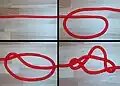
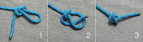
    1. Form an overhand noose, or simply tie an overhand knot around the standing part as shown.
    2. Tighten the overhand portion of the knot around the standing part. Thread the working part through the loop.
    3. First close the noose on the working part by pulling on the standing part, then remove any remaining slack in the knot by pulling on the working part. The knot should have a tidy, triangular shape where the standing part enters the knot. (See image at right.)

    See also

    References

    1. Ashley, Clifford W. (1944). The Ashley Book of Knots. Doubleday & Company. p. 7 & 86. ISBN 0-385-04025-3. {{cite book}}: ISBN / Date incompatibility (help)
    2. Ashley, Clifford W. (1944). The Ashley Book of Knots, p.86. Doubleday. ISBN 0-385-04025-3.

    Further reading

    • Budworth, Geoffrey (2001). The Ultimate Encyclopedia of Knots & Ropework. Anness Publishing LTD. ISBN 9781859679111.

    This article is adapted from “Ashley's stopper knot” on Wikipedia, written by its contributors, and used under CC BY-SA 4.0. Text on this page is available under the same licence. Source snapshot: Wikipedia via Kiwix, 2026-07-20.

  • Ashley’s bend

    Ashley’s Bend
    Ashley's bend
    Names Ashley’s Bend, Ashley bend
    Category Bend
    Origin The Ashley Book of Knots
    Related Alpine butterfly bend, Hunter’s bend, Zeppelin bend, Butterfly loop, Trident loop
    Releasing Jamming possible
    Typical use temporary joining of similar-sized cords & ropes
    ABoK #1452, #1408

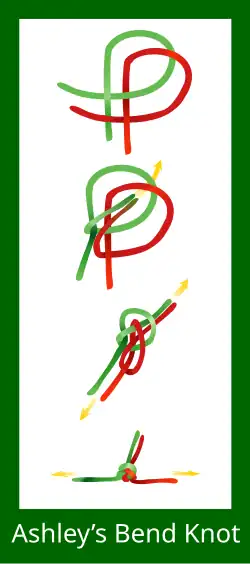
    Ashley’s bend is a knot used to securely join the ends of two ropes together. It is similar to several related bend knots which consist of two interlocking overhand knots, and in particular the alpine butterfly bend.[1] These related bends differ by the way the two constituent overhand knots are interlocked.

    History

    The name “Ashley’s bend” is now associated with the knot described in entry #1452 of The Ashley Book of Knots. Clifford Ashley developed this bend and believed it to be original, along with several similar ones. Rather than giving it a name he simply noted the date when he first tied it: “(2/3/34.)”.[2] Cyrus L. Day, a contemporary of Ashley’s, called the knot by the name “Ashley’s Bend” in his 1947 book The Art of Knotting & Splicing just a few years after the publication of Ashley’s book.[3][4] Later authors have continued to use this name.[5][6]

    Security

    In the 1930s, Ashley performed security tests on a number of bends for the Collins and Aikman company.[7] The manufacturer wanted a bend that would not slip when tied in mohair, a stiff slippery material. The jerk testing Ashley performed placed his bend, #1452, equal to the barrel knot in exhibiting no slippage at all. All other bends he tested slipped to some extent, and most failed completely in less than 100 loading cycles.[8]

    Jamming behavior

    Most references fail to distinguish the distinct ways in which the two ends of the knot can be dressed. As the two working ends emerge from the knot, they make a sort of vortex that twists the tails in one direction; the tails can be oriented such that they are twisted ever tighter together, or put on the other side of each other in which case the setting of the knot can lead to a jamming state.

    Uses

    This knot belongs to a group of knots formed by interlocking overhand knots. Its purpose is to securely join two ropes of similar thickness. Ashley’s testing confirmed its reliability with minimal slipping tendencies. One needs to dress the knot correctly for easy loosening when expecting a heavy load.

    See also

    Notes and references

    1. “Ashley’s Bend | How tie the Ashley’s Bend Knot | All knots animated”. www.netknots.com. Retrieved 2024-05-14.
    2. Ashley, Clifford W. (1944). The Ashley Book of Knots. New York: Doubleday. p. 264. 1452. (2/3/34.) Another original bend that is as easily untied as #1451. It appears to be strong, secure and compact…
    3. Day, Cyrus Lawrence (1947), The Art of Knotting and Splicing (1st ed.), New York: Dodd, Mead & Co., pp. 64–65
    4. The name “Ashley’s Bend” is only used in the index (p. 223) of the first edition (1947) of The Art of Knotting and Splicing, not the main discussion of the knot on page 64. By the second edition (1955) the name also appears in the main text.
    5. Pawson, Des (2002). Pocket Guide to Knots & Splices. Edison, NJ: Chartwell Books. pp. 124–125.
    6. Perry, Gordon (2006). Knots. Vancouver, BC: Whitecap Books. p. 78.
    7. Ashley, pp. 16–17
    8. Ashley, p. 273

    This article is adapted from “Ashley's bend” on Wikipedia, written by its contributors, and used under CC BY-SA 4.0. Text on this page is available under the same licence. Source snapshot: Wikipedia via Kiwix, 2026-07-20.

  • Open knot theory

    The theory of open knots attempts to describe entanglements in open curves or filaments in a mathematically consistent way and develop tools and algorithms which can categorize the topology of an open curve. In the mathematical field of knot theory, knots are only considered in closed loops. What is colloquially considered a knot, for example a piece of rope tied into an overhand knot, would not be considered a mathematical knot unless the two ends of the rope were connected. Research into open knot theory is motivated by a desire to understand the formation and properties of knots in proteins and DNA molecules, which often do not form closed loops, and to draw closer connections between knot theory and the properties of physical knots.

    Connecting the ends of a knot
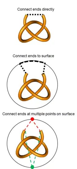
    An open entangled curve virtually closed. If the ends are connected directly or to two close points on an enclosing sphere, the curve can be classified as a trefoil knot. If the ends are connected to other points on the sphere, the curve may be an unknot (green) or a trefoil (red).

    Virtual closure

    Drawing a straight line from one end of a curve to another effectively closes it into a loop. After this virtual closure, the knot can be classified by computing an invariant such as the Alexander polynomial. If the two ends of a knotted curve filament are close to each other or well separated from the highly knotted portion, this direct virtual closure will not introduce new crossings into a diagram. However, there are configurations where direct closure can virtually turn a knot into a slipknot and effectively erase the knot, or introduce additional complexity that is not present in the initial curve. In such cases, it may be beneficial to connect the ends of the curve by virtual lines to an external surface enclosing the curve, such as a sphere with a large radius, and then connecting the ends of two lines along the surface so that they do not interfere with the curve itself. An algorithm known as minimally interfering closure will determine whether the two ends of an open polygonal knot are closer to each other or to the convex hull of the knot, and connect them by whichever path is shorter.[1]

    The choice of virtual closure scheme will influence which type of knot a curve is determined to be consistent with. A more general method known as stochastic closure chooses many uniformly distributed points on the surface of a large sphere enclosing the curve and connects the ends to each of those points and computes the knot type at each closure. This yields a distribution of different knot types at different regions around the sphere which can be visualized as a map.[2] This is primarily used for analyzing knotted proteins.

    knotoid diagrams
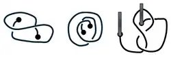
    Three knotoid diagrams, two with two crossings and one with three crossings. The ends of the three-crossing knotoid are shown with pegs, to demonstrate that the curve cannot be passed over them.

    Knotoids and virtual knots

    Rather than attempting to map an open curve onto a specific closed knot, concepts have been developed to classify open entanglements. One such concept is the knotoid which is a generalization of a knot diagram which includes the two ends of the curve, first described by Turaev in 2010.[3] When a Reidemeister move is applied to a diagram of a knot, the knot topology cannot change. If a Reidemeister move on a knotoid diagram moves part of the curve over one of the ends, it will change the type of knotoid and is considered “forbidden.” In this sense, a knotoid can be envisioned as a knotted piece of string on ground with its ends attached to two vertical pegs; the knotoid type will not change unless the string is lifted and unwrapped around the pegs. Like knots, knotoids can be classified based on their crossing number, and invariants such as polynomials have been derived to distinguish them. An open curve in three dimensions will be consistent with different knotoids depending on the surface that it is projected onto. Similar to stochastic closure, the full picture of a curve’s topological complexity must be determined by sampling the knotoids of many projections. It is possible to compute the minimum number of “forbidden” knotoid moves (passing a curve in the diagram over one of the ends) to reach a trivial crossing-free knotoid,[4] which provides a measure of complexity of an open curve similar to the unknotting number.

    Virtual knots are another generalization of knot diagrams. Whereas knotoids deal with ambiguous closure, virtual knots deal with ambiguous crossings. Where one part of a knot diagram passes over or under another, two parts of a virtual knot diagram may meet at a point, called a virtual crossing. A diagram of an open knot may be treated as a virtual knot by connecting its to ends with a line and creating a virtual crossing at each point the end intersects the diagram.

    Extension of knot invariants

    Definitions of knot invariants that categorize the topology of closed curves can be generalized to describe open curves. An example is the space writhe which is an extension of the Gauss linking number, and describes how many times a curve will cross over itself when viewed from different directions.[5] More entangled and twisted curves will typically have a higher space writhe, however an unentangled curve such as a helix will also have a high space writhe. Similarly, the Gauss linking integral can be computed from two open curves, such as two strands in a hair braid, to determine how many times one curve winds around another. Other knot invariants have also been extended to open curves, including the second Vassiliev invariant[6] and the Jones polynomial.[7]

    Applications

    Many of the techniques used to categorize open entangled curves have been applied to the study of knotted proteins. This includes a categorization of knotted protein structures based on stochastic closure,[2] using knotoids,[4] virtual knots,[8] the space writhe,[9] and open versions of the second Vassiliev invariant [10] and Jones polynomial.[11] Beyond simply categorization, a goal of this research is to understand the formation and stability of these knotted proteins. Similar analysis has also been applied to DNA, which does not have a stable native state like proteins do. The most common tool used to determine the topology of simulated DNA molecules is the Alexander molecule combined with chain closure, which has been used to detect knots in simulated DNA in virus capsids,[12] human chromosomes,[13] as well as simpler models of polymers,[14] of which DNA is an example. Beyond the study of biomolecules, tools from open knot theory have been applied to physical ropes, for example in determining the most effective way to tie two pieces of rope together by comparing the writhe within each type of knot to the force required to pull two tied ropes apart.[15]

    References

    1. Tubiana, Luca; Orlandini, Enzo; Micheletti, Cristian (2011). “Probing the Entanglement and Locating Knots in Ring Polymers: A Comparative Study of Different Arc Closure Schemes” (PDF). Progress of Theoretical Physics Supplement. 191: 192–204. arXiv:1103.0475. Bibcode:2011PThPS.191..192T. doi:10.1143/ptps.191.192. ISSN 0375-9687. Retrieved 2025-09-21.
    2. 1 2 Mansfield, Marc L. (1994). “Are there knots in proteins?”. Nature Structural & Molecular Biology. 1 (4): 213–214. doi:10.1038/nsb0494-213. ISSN 1545-9993. PMID 7656045.
    3. Turaev, Vladimir (2010). “Knotoids”. arXiv:1002.4133 [math.GT].
    4. 1 2 Barbensi, Agnese; Goundaroulis, Dimos (2021). “f -distance of knotoids and protein structure”. Proceedings of the Royal Society A: Mathematical, Physical and Engineering Sciences. 477 (2246) 20200898. arXiv:1909.08556. Bibcode:2021RSPSA.47700898B. doi:10.1098/rspa.2020.0898. ISSN 1364-5021.
    5. Berger, Mitchell A; Prior, Chris (2006-06-30). “The writhe of open and closed curves”. Journal of Physics A: Mathematical and General. 39 (26): 8321–8348. Bibcode:2006JPhA…39.8321B. doi:10.1088/0305-4470/39/26/005. ISSN 0305-4470. Retrieved 2025-09-21.
    6. Panagiotou, Eleni; Kauffman, Louis H. (2021). “Vassiliev measures of complexity of open and closed curves in 3-space”. Proceedings of the Royal Society A: Mathematical, Physical and Engineering Sciences. 477 (2254) 20210440. arXiv:2104.12275. Bibcode:2021RSPSA.47710440P. doi:10.1098/rspa.2021.0440. ISSN 1364-5021.
    7. Panagiotou, Eleni; Kauffman, Louis H. (2020). “Knot polynomials of open and closed curves”. Proceedings of the Royal Society A: Mathematical, Physical and Engineering Sciences. 476 (2240) 20200124. arXiv:2001.01303. Bibcode:2020RSPSA.47600124P. doi:10.1098/rspa.2020.0124. ISSN 1364-5021. PMC 7482204. PMID 32922152.
    8. Alexander, Keith; Taylor, Alexander J.; Dennis, Mark R. (2017-02-13). “Proteins analysed as virtual knots” (PDF). Scientific Reports. 7 (1) 42300. arXiv:1611.06185. Bibcode:2017NatSR…742300A. doi:10.1038/srep42300. ISSN 2045-2322. PMC 5304221. PMID 28205562. Retrieved 2025-09-21.
    9. Røgen, Peter; Fain, Boris (2003-01-07). “Automatic classification of protein structure by using Gauss integrals”. Proceedings of the National Academy of Sciences. 100 (1): 119–124. Bibcode:2003PNAS..100..119R. doi:10.1073/pnas.2636460100. ISSN 0027-8424. PMC 140900. PMID 12506205.
    10. Wang, Jason; Panagiotou, Eleni (2022-04-16). “The protein folding rate and the geometry and topology of the native state” (PDF). Scientific Reports. 12 (1) 6384. Bibcode:2022NatSR..12.6384W. doi:10.1038/s41598-022-09924-0. ISSN 2045-2322. PMC 9013383. PMID 35430582. Retrieved 2025-09-21.
    11. Song, Ruzhi; Li, Fengling; Wu, Jie; Lei, Fengchun; Wei, Guo-Wei (2025). “Multi-scale Jones polynomial and persistent Jones polynomial for knot data analysis”. AIMS Mathematics. 10 (1): 1463–1487. doi:10.3934/math.2025068. ISSN 2473-6988. PMC 12363994. PMID 40838040.
    12. Arsuaga, Javier; Vazquez, Mariel; McGuirk, Paul; Trigueros, Sonia; Sumners, De Witt; Roca, Joaquim (2005-06-28). “DNA knots reveal a chiral organization of DNA in phage capsids”. Proceedings of the National Academy of Sciences. 102 (26): 9165–9169. Bibcode:2005PNAS..102.9165A. doi:10.1073/pnas.0409323102. ISSN 0027-8424. PMC 1166588. PMID 15958528.
    13. Siebert, Jonathan; Kivel, Alexey; Atkinson, Liam; Stevens, Tim; Laue, Ernest; Virnau, Peter (2017-08-02). “Are There Knots in Chromosomes?”. Polymers. 9 (8): 317. doi:10.3390/polym9080317. ISSN 2073-4360. PMC 6418659. PMID 30971010.
    14. Tubiana, L.; Rosa, A.; Fragiacomo, F.; Micheletti, C. (2013-05-14). “Spontaneous Knotting and Unknotting of Flexible Linear Polymers: Equilibrium and Kinetic Aspects”. Macromolecules. 46 (9): 3669–3678. arXiv:1304.3470. Bibcode:2013MaMol..46.3669T. doi:10.1021/ma4002963. ISSN 0024-9297.
    15. Patil, Vishal P.; Sandt, Joseph D.; Kolle, Mathias; Dunkel, Jörn (2020-01-03). “Topological mechanics of knots and tangles”. Science. 367 (6473): 71–75. Bibcode:2020Sci…367…71P. doi:10.1126/science.aaz0135. ISSN 0036-8075. PMID 31896713.

    This article is adapted from “Open knot theory” on Wikipedia, written by its contributors, and used under CC BY-SA 4.0. Text on this page is available under the same licence. Source snapshot: Wikipedia via Kiwix, 2026-07-20.

  • Artin–Tits group

    In the mathematical area of group theory, Artin groups, also known as Artin–Tits groups or generalized braid groups, are a family of infinite discrete groups defined by simple presentations. They are closely related with Coxeter groups. Examples are free groups, free abelian groups, braid groups, and right-angled Artin–Tits groups, among others.

    The groups are named after Emil Artin, due to his early work on braid groups in the 1920s to 1940s,[1] and Jacques Tits who developed the theory of a more general class of groups in the 1960s.[2]

    Definition

    An Artin–Tits presentation is a group presentation S R {\displaystyle \langle S\mid R\rangle } {\displaystyle \langle S\mid R\rangle } where S {\displaystyle S} {\displaystyle S} is a (usually finite) set of generators and R {\displaystyle R} {\displaystyle R} is a set of Artin–Tits relations, namely relations of the form s t s t = t s t s {\displaystyle stst\ldots =tsts\ldots } {\displaystyle stst\ldots =tsts\ldots } for distinct s , t {\displaystyle s,t} {\displaystyle s,t} in S {\displaystyle S} {\displaystyle S}, where both sides have equal lengths, and there exists at most one relation for each pair of distinct generators s , t {\displaystyle s,t} {\displaystyle s,t}. An Artin–Tits group is a group that admits an Artin–Tits presentation. Likewise, an Artin–Tits monoid is a monoid that, as a monoid, admits an Artin–Tits presentation.

    Alternatively, an Artin–Tits group can be specified by the set of generators S {\displaystyle S} {\displaystyle S} and, for every s , t {\displaystyle s,t} {\displaystyle s,t} in S {\displaystyle S} {\displaystyle S}, the natural number m s , t 2 {\displaystyle m_{s,t}\geqslant 2} {\displaystyle m_{s,t}\geqslant 2} that is the length of the words s t s t {\displaystyle stst\ldots } {\displaystyle stst\ldots } and t s t s {\displaystyle tsts\ldots } {\displaystyle tsts\ldots } such that s t s t = t s t s {\displaystyle stst\ldots =tsts\ldots } {\displaystyle stst\ldots =tsts\ldots } is the relation connecting s {\displaystyle s} {\displaystyle s} and t {\displaystyle t} {\displaystyle t}, if any. By convention, one puts m s , t = {\displaystyle m_{s,t}=\infty } {\displaystyle m_{s,t}=\infty } when there is no relation s t s t = t s t s {\displaystyle stst\ldots =tsts\ldots } {\displaystyle stst\ldots =tsts\ldots } . Formally, if we define s , t m {\displaystyle \langle s,t\rangle ^{m}} {\displaystyle \langle s,t\rangle ^{m}} to denote an alternating product of s {\displaystyle s} {\displaystyle s} and t {\displaystyle t} {\displaystyle t} of length m {\displaystyle m} {\displaystyle m}, beginning with s {\displaystyle s} {\displaystyle s} — so that s , t 2 = s t {\displaystyle \langle s,t\rangle ^{2}=st} {\displaystyle \langle s,t\rangle ^{2}=st}, s , t 3 = s t s {\displaystyle \langle s,t\rangle ^{3}=sts} {\displaystyle \langle s,t\rangle ^{3}=sts}, etc. — the Artin–Tits relations take the form

    s , t m s , t = t , s m t , s ,  where  m s , t = m t , s { 2 , 3 , , } . {\displaystyle \langle s,t\rangle ^{m_{s,t}}=\langle t,s\rangle ^{m_{t,s}},{\text{ where }}m_{s,t}=m_{t,s}\in \{2,3,\ldots ,\infty \}.} {\displaystyle \langle s,t\rangle ^{m_{s,t}}=\langle t,s\rangle ^{m_{t,s}},{\text{ where }}m_{s,t}=m_{t,s}\in \{2,3,\ldots ,\infty \}.}

    The integers m s , t {\displaystyle m_{s,t}} {\displaystyle m_{s,t}} can be organized into a symmetric matrix, known as the Coxeter matrix of the group.

    If S R {\displaystyle \langle S\mid R\rangle } {\displaystyle \langle S\mid R\rangle } is an Artin–Tits presentation of an Artin–Tits group A {\displaystyle A} {\displaystyle A}, the quotient of A {\displaystyle A} {\displaystyle A} obtained by adding the relation s 2 = 1 {\displaystyle s^{2}=1} {\displaystyle s^{2}=1} for each s {\displaystyle s} {\displaystyle s} of R {\displaystyle R} {\displaystyle R} is a Coxeter group. Conversely, if W {\displaystyle W} {\displaystyle W} is a Coxeter group presented by reflections and the relations s 2 = 1 {\displaystyle s^{2}=1} {\displaystyle s^{2}=1} are removed, the extension thus obtained is an Artin–Tits group. For instance, the Coxeter group associated with the n {\displaystyle n} {\displaystyle n}-strand braid group is the symmetric group of all permutations of { 1 , , n } {\displaystyle \{1,\ldots ,n\}} {\displaystyle \{1,\ldots ,n\}}.

    Examples

    • G = S {\displaystyle G=\langle S\mid \emptyset \rangle } {\displaystyle G=\langle S\mid \emptyset \rangle } is the free group based on S {\displaystyle S} {\displaystyle S}; here m s , t = {\displaystyle m_{s,t}=\infty } {\displaystyle m_{s,t}=\infty } for all s , t {\displaystyle s,t} {\displaystyle s,t}.
    • G = S { s t = t s s , t S } {\displaystyle G=\langle S\mid \{st=ts\mid s,t\in S\}\rangle } {\displaystyle G=\langle S\mid \{st=ts\mid s,t\in S\}\rangle } is the free abelian group based on S {\displaystyle S} {\displaystyle S}; here m s , t = 2 {\displaystyle m_{s,t}=2} {\displaystyle m_{s,t}=2} for all s , t {\displaystyle s,t} {\displaystyle s,t}.
    • G = σ 1 , , σ n 1 σ i σ j σ i = σ j σ i σ j  for  | i j | = 1 , σ i σ j = σ j σ i  for  | i j | 2 {\displaystyle G=\langle \sigma _{1},\ldots ,\sigma _{n-1}\mid \sigma _{i}\sigma _{j}\sigma _{i}=\sigma _{j}\sigma _{i}\sigma _{j}{\text{ for }}\vert i-j\vert =1,\sigma _{i}\sigma _{j}=\sigma _{j}\sigma _{i}{\text{ for }}\vert i-j\vert \geqslant 2\rangle } {\displaystyle G=\langle \sigma _{1},\ldots ,\sigma _{n-1}\mid \sigma _{i}\sigma _{j}\sigma _{i}=\sigma _{j}\sigma _{i}\sigma _{j}{\text{ for }}\vert i-j\vert =1,\sigma _{i}\sigma _{j}=\sigma _{j}\sigma _{i}{\text{ for }}\vert i-j\vert \geqslant 2\rangle } is the braid group on n {\displaystyle n} {\displaystyle n} strands; here m σ i , σ j = 3 {\displaystyle m_{\sigma _{i},\sigma _{j}}=3} {\displaystyle m_{\sigma _{i},\sigma _{j}}=3} for | i j | = 1 {\displaystyle \vert i-j\vert =1} {\displaystyle \vert i-j\vert =1}, and m σ i , σ j = 2 {\displaystyle m_{\sigma _{i},\sigma _{j}}=2} {\displaystyle m_{\sigma _{i},\sigma _{j}}=2} for | i j | > 1 {\displaystyle \vert i-j\vert >1} {\displaystyle \vert i-j\vert >1}.

    General properties

    Artin–Tits monoids are eligible for Garside methods based on the investigation of their divisibility relations, and are well understood:

    • Artin–Tits monoids are cancellative, and they admit greatest common divisors and conditional least common multiples (a least common multiple exists whenever a common multiple does).
    • If A + {\displaystyle A^{+}} {\displaystyle A^{+}} is an Artin–Tits monoid, and if W {\displaystyle W} {\displaystyle W} is the associated Coxeter group, there is a (set-theoretic) section σ {\displaystyle \sigma } {\displaystyle \sigma } of W {\displaystyle W} {\displaystyle W} into A + {\displaystyle A^{+}} {\displaystyle A^{+}}, and every element of A + {\displaystyle A^{+}} {\displaystyle A^{+}} admits a distinguished decomposition as a sequence of elements in the image of σ {\displaystyle \sigma } {\displaystyle \sigma } (“greedy normal form”).

    Very few results are known for general Artin–Tits groups. In particular, the following basic questions remain open in the general case:

    – solving the word and conjugacy problems — which are conjectured to be decidable,
    – determining torsion — which is conjectured to be trivial,
    – determining the center — which is conjectured to be trivial or monogenic in the case when the group is not a direct product (“irreducible case”),
    – determining the cohomology — in particular solving the K ( π , 1 ) {\displaystyle K(\pi ,1)} {\displaystyle K(\pi ,1)} conjecture, i.e., finding an acyclic complex whose fundamental group is the considered group.

    Partial results involving particular subfamilies are gathered below. Among the few known general results, one can mention:

    • Artin–Tits groups are infinite countable.
    • In an Artin–Tits group S R {\displaystyle \langle S\mid R\rangle } {\displaystyle \langle S\mid R\rangle }, the only relation connecting the squares of the elements s , t {\displaystyle s,t} {\displaystyle s,t} of S {\displaystyle S} {\displaystyle S} is s 2 t 2 = t 2 s 2 {\displaystyle s^{2}t^{2}=t^{2}s^{2}} {\displaystyle s^{2}t^{2}=t^{2}s^{2}} if s t = t s {\displaystyle st=ts} {\displaystyle st=ts} is in R {\displaystyle R} {\displaystyle R} (John Crisp and Luis Paris [3]).
    • For every Artin–Tits presentation S R {\displaystyle \langle S\mid R\rangle } {\displaystyle \langle S\mid R\rangle }, the Artin–Tits monoid presented by S R {\displaystyle \langle S\mid R\rangle } {\displaystyle \langle S\mid R\rangle } embeds in the Artin–Tits group presented by S R {\displaystyle \langle S\mid R\rangle } {\displaystyle \langle S\mid R\rangle } (Paris[4]).
    • Every (finitely generated) Artin–Tits monoid admits a finite Garside family (Matthew Dyer and Christophe Hohlweg[5]). As a consequence, the existence of common right-multiples in Artin–Tits monoids is decidable, and reduction of multifractions is effective.

    Particular classes of Artin–Tits groups

    Several important classes of Artin groups can be defined in terms of the properties of the Coxeter matrix.

    Artin–Tits groups of spherical type

    • An Artin–Tits group is said to be of spherical type if the associated Coxeter group W {\displaystyle W} {\displaystyle W} is finite — the alternative terminology “Artin–Tits group of finite type” is to be avoided, because of its ambiguity: a “finite type group” is just one that admits a finite generating set. Recall that a complete classification is known, the ‘irreducible types’ being labeled as the infinite series A n {\displaystyle A_{n}} {\displaystyle A_{n}}, B n {\displaystyle B_{n}} {\displaystyle B_{n}}, D n {\displaystyle D_{n}} {\displaystyle D_{n}}, I 2 ( n ) {\displaystyle I_{2}(n)} {\displaystyle I_{2}(n)} and six exceptional groups E 6 {\displaystyle E_{6}} {\displaystyle E_{6}}, E 7 {\displaystyle E_{7}} {\displaystyle E_{7}}, E 8 {\displaystyle E_{8}} {\displaystyle E_{8}}, F 4 {\displaystyle F_{4}} {\displaystyle F_{4}}, H 3 {\displaystyle H_{3}} {\displaystyle H_{3}}, and H 4 {\displaystyle H_{4}} {\displaystyle H_{4}}.
    • In the case of a spherical Artin–Tits group, the group is a group of fractions for the monoid, making the study much easier. Every above-mentioned problem is solved in the positive for spherical Artin–Tits groups: the word and conjugacy problems are decidable, their torsion is trivial, the center is monogenic in the irreducible case, and the cohomology is determined (Pierre Deligne, by geometrical methods,[6] Egbert Brieskorn and Kyoji Saito, by combinatorial methods [7]).
    • A pure Artin–Tits group of spherical type can be realized as the fundamental group of the complement of a finite hyperplane arrangement in C n {\displaystyle \mathbb {C} ^{n}} {\displaystyle \mathbb {C} ^{n}}.
    • Artin–Tits groups of spherical type are biautomatic groups (Ruth Charney[8]).
    • In modern terminology, an Artin–Tits group A {\displaystyle A} {\displaystyle A} is a Garside group, meaning that A {\displaystyle A} {\displaystyle A} is a group of fractions for the associated monoid A + {\displaystyle A^{+}} {\displaystyle A^{+}} and there exists for each element of A {\displaystyle A} {\displaystyle A} a unique normal form that consists of a finite sequence of (copies of) elements of W {\displaystyle W} {\displaystyle W} and their inverses (“symmetric greedy normal form”)

    Right-angled Artin groups

    • An Artin–Tits group is said to be right-angled if all coefficients of the Coxeter matrix are either 2 {\displaystyle 2} {\displaystyle 2} or {\displaystyle \infty } {\displaystyle \infty }, i.e., all relations are commutation relations s t = t s {\displaystyle st=ts} {\displaystyle st=ts}. The names (free) partially commutative group, graph group, trace group, semifree group or even locally free group are also common.
    • For this class of Artin–Tits groups, a different labeling scheme is commonly used. Any graph Γ {\displaystyle \Gamma } {\displaystyle \Gamma } on n {\displaystyle n} {\displaystyle n} vertices labeled 1 , 2 , , n {\displaystyle 1,2,\ldots ,n} {\displaystyle 1,2,\ldots ,n} defines a matrix M {\displaystyle M} {\displaystyle M}, for which m s , t = 2 {\displaystyle m_{s,t}=2} {\displaystyle m_{s,t}=2} if the vertices s {\displaystyle s} {\displaystyle s} and t {\displaystyle t} {\displaystyle t} are connected by an edge in Γ {\displaystyle \Gamma } {\displaystyle \Gamma }, and m s , t = {\displaystyle m_{s,t}=\infty } {\displaystyle m_{s,t}=\infty } otherwise.
    • The class of right-angled Artin–Tits groups includes the free groups of finite rank, corresponding to a graph with no edges, and the finitely-generated free abelian groups, corresponding to a complete graph. Every right-angled Artin group of rank r can be constructed as HNN extension of a right-angled Artin group of rank r 1 {\displaystyle r-1} {\displaystyle r-1}, with the free product and direct product as the extreme cases. A generalization of this construction is called a graph product of groups. A right-angled Artin group is a special case of this product, with every vertex/operand of the graph-product being a free group of rank one (the infinite cyclic group).
    • The word and conjugacy problems of a right-angled Artin–Tits group are decidable, the former in linear time, the group is torsion-free, and there is an explicit cellular finite K ( π , 1 ) {\displaystyle K(\pi ,1)} {\displaystyle K(\pi ,1)} (John Crisp, Eddy Godelle, and Bert Wiest[9]).
    • Every right-angled Artin–Tits group acts freely and cocompactly on a finite-dimensional CAT(0) cube complex, its “Salvetti complex”. As an application, one can use right-angled Artin groups and their Salvetti complexes to construct groups with given finiteness properties (Mladen Bestvina and Noel Brady [10]) see also (Ian Leary [11]).

    Artin–Tits groups of large type

    • An Artin–Tits group (and a Coxeter group) is said to be of large type if m s , t 3 {\displaystyle m_{s,t}\geqslant 3} {\displaystyle m_{s,t}\geqslant 3} for all generators s t {\displaystyle s\neq t} {\displaystyle s\neq t}; it is said to be of extra-large type if m s , t 4 {\displaystyle m_{s,t}\geqslant 4} {\displaystyle m_{s,t}\geqslant 4} for all generators s t {\displaystyle s\neq t} {\displaystyle s\neq t}.
    • Artin–Tits groups of extra-large type are eligible for small cancellation theory. As an application, Artin–Tits groups of extra-large type are torsion-free and have solvable conjugacy problem (Kenneth Appel and Paul Schupp[12]).
    • Artin–Tits groups of extra-large type are biautomatic (David Peifer[13]).
    • Artin groups of large type are shortlex automatic with regular geodesics (Derek Holt and Sarah Rees[14]).

    Other types

    Many other families of Artin–Tits groups have been identified and investigated. Here we mention two of them.

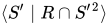
    • An Artin–Tits group S R {\displaystyle \langle S\mid R\rangle } {\displaystyle \langle S\mid R\rangle } is said to be of FC type (“flag complex”) if, for every subset S {\displaystyle S’} {\displaystyle S'} of S {\displaystyle S} {\displaystyle S} such that m s , t {\displaystyle m_{s,t}\neq \infty } {\displaystyle m_{s,t}\neq \infty } for all s , t {\displaystyle s,t} {\displaystyle s,t} in S {\displaystyle S’} {\displaystyle S'}, the group S R S 2 {\displaystyle \langle S’\mid R\cap S'{}^{2}\rangle } {\displaystyle \langle S'\mid R\cap S'{}^{2}\rangle } is of spherical type. Such groups act cocompactly on a CAT(0) cubical complex, and, as a consequence, one can find a rational normal form for their elements and deduce a solution to the word problem (Joe Altobelli and Charney [15]). An alternative normal form is provided by multifraction reduction, which gives a unique expression by an irreducible multifraction directly extending the expression by an irreducible fraction in the spherical case (Dehornoy[16]).
    • An Artin–Tits group is said to be of affine type if the associated Coxeter group is affine. They correspond to the extended Dynkin diagrams of the four infinite families A ~ n {\displaystyle {\widetilde {A}}_{n}} {\displaystyle {\widetilde {A}}_{n}} for n 1 {\displaystyle n\geqslant 1} {\displaystyle n\geqslant 1}, B ~ n {\displaystyle {\widetilde {B}}_{n}} {\displaystyle {\widetilde {B}}_{n}}, C ~ n {\displaystyle {\widetilde {C}}_{n}} {\displaystyle {\widetilde {C}}_{n}} for n 2 {\displaystyle n\geqslant 2} {\displaystyle n\geqslant 2}, and D ~ n {\displaystyle {\widetilde {D}}_{n}} {\displaystyle {\widetilde {D}}_{n}} for n 3 {\displaystyle n\geqslant 3} {\displaystyle n\geqslant 3}, and of the five sporadic types E ~ 6 {\displaystyle {\widetilde {E}}_{6}} {\displaystyle {\widetilde {E}}_{6}}, E ~ 7 {\displaystyle {\widetilde {E}}_{7}} {\displaystyle {\widetilde {E}}_{7}}, E ~ 8 {\displaystyle {\widetilde {E}}_{8}} {\displaystyle {\widetilde {E}}_{8}}, F ~ 4 {\displaystyle {\widetilde {F}}_{4}} {\displaystyle {\widetilde {F}}_{4}}, and G ~ 2 {\displaystyle {\widetilde {G}}_{2}} {\displaystyle {\widetilde {G}}_{2}}. Affine Artin–Tits groups are of Euclidean type: the associated Coxeter group acts geometrically on a Euclidean space. As a consequence, their center is trivial, and their word problem is decidable (Jon McCammond and Robert Sulway [17]). In 2019, a proof of the K ( π , 1 ) {\displaystyle K(\pi ,1)} {\displaystyle K(\pi ,1)} conjecture was announced for all affine Artin–Tits groups (Mario Salvetti and Giovanni Paolini[18]).

    See also

    • Free partially commutative monoid
    • Artinian group (an unrelated notion)
    • Non-commutative cryptography
    • Elementary abelian group

    References

    1. Artin, Emil (1947). “Theory of Braids”. Annals of Mathematics. 48 (1): 101–126. doi:10.2307/1969218. JSTOR 1969218. S2CID 30514042.
    2. Tits, Jacques (1966), “Normalisateurs de tores. I. Groupes de Coxeter étendus”, Journal of Algebra, 4: 96–116, doi:10.1016/0021-8693(66)90053-6, MR 0206117
    3. Crisp, John; Paris, Luis (2001), “The solution to a conjecture of Tits on the subgroup generated by the squares of the generators of an Artin group”, Inventiones Mathematicae, 145 (1): 19–36, arXiv:math/0003133, Bibcode:2001InMat.145…19C, doi:10.1007/s002220100138, MR 1839284
    4. Paris, Luis (2002), “Artin monoids inject in their groups”, Commentarii Mathematici Helvetici, 77 (3): 609–637, arXiv:math/0102002, doi:10.1007/s00014-002-8353-z, MR 1933791
    5. Dyer, Matthew; Hohlweg, Christophe (2016), “Small roots, low elements, and the weak order in Coxeter groups”, Advances in Mathematics, 301: 739–784, arXiv:1505.02058, doi:10.1016/j.aim.2016.06.022, MR 1839284
    6. Deligne, Pierre (1972), “Les immeubles des groupes de tresses généralisés”, Inventiones Mathematicae, 17 (4): 273–302, Bibcode:1972InMat..17..273D, doi:10.1007/BF01406236, MR 0422673
    7. Brieskorn, Egbert; Saito, Kyoji (1972), “Artin-Gruppen und Coxeter-Gruppen”, Inventiones Mathematicae, 17 (4): 245–271, Bibcode:1972InMat..17..245B, doi:10.1007/BF01406235, MR 0323910
    8. Charney, Ruth (1992), “Artin groups of finite type are biautomatic”, Mathematische Annalen, 292 (4): 671–683, doi:10.1007/BF01444642, MR 1157320
    9. Crisp, John; Godelle, Eddy; Wiest, Bert (2009), “The conjugacy problem in subgroups of right-angled Artin groups”, Journal of Topology, 2 (3): 442–460, doi:10.1112/jtopol/jtp018, MR 2546582
    10. Bestvina, Mladen; Brady, Noel (1997), “Morse theory and finiteness properties of groups”, Inventiones Mathematicae, 129 (3): 445–470, Bibcode:1997InMat.129..445B, doi:10.1007/s002220050168, MR 1465330
    11. Leary, Ian (2018), “Uncountably many groups of type FP”, Proceedings of the London Mathematical Society, 117 (2): 246–276, arXiv:1512.06609, doi:10.1112/plms.12135, MR 3851323
    12. Appel, Kenneth I.; Schupp, Paul E. (1983), “Artin Groups and Infinite Coxeter Groups”, Inventiones Mathematicae, 72 (2): 201–220, Bibcode:1983InMat..72..201A, doi:10.1007/BF01389320, MR 0700768
    13. Peifer, David (1996), “Artin groups of extra-large type are biautomatic”, Journal of Pure and Applied Algebra, 110 (1): 15–56, doi:10.1016/0022-4049(95)00094-1, MR 1390670
    14. Holt, Derek; Rees, Sarah (2012). “Artin groups of large type are shortlex automatic with regular geodesics”. Proceedings of the London Mathematical Society. 104 (3): 486–512. arXiv:1003.6007. doi:10.1112/plms/pdr035. MR 2900234.
    15. Altobelli, Joe; Charney, Ruth (2000), “A geometric rational form for Artin groups of FC type”, Geometriae Dedicata, 79 (3): 277–289, doi:10.1023/A:1005216814166, MR 1755729
    16. Dehornoy, Patrick (2017), “Multifraction reduction I: The 3-Ore case and Artin–Tits groups of type FC”, Journal of Combinatorial Algebra, 1 (2): 185–228, arXiv:1606.08991, doi:10.4171/JCA/1-2-3, MR 3634782
    17. McCammond, Jon; Sulway, Robert (2017), “Artin groups of Euclidean type”, Inventiones Mathematicae, 210 (1): 231–282, arXiv:1312.7770, Bibcode:2017InMat.210..231M, doi:10.1007/s00222-017-0728-2, MR 3698343
    18. Paolini, Giovanni; Salvetti, Mario (2019), “Proof of the K ( π , 1 ) {\displaystyle K(\pi ,1)} {\displaystyle K(\pi ,1)} conjecture for affine Artin groups”, Inventiones Mathematicae, 224 (2): 487–572, arXiv:1907.11795, doi:10.1007/s00222-020-01016-y

    Further reading

    • Charney, Ruth (2007), “An introduction to right-angled Artin groups”, Geometriae Dedicata, 125 (1): 141–158, arXiv:math/0610668, doi:10.1007/s10711-007-9148-6, MR 2322545
    • Godelle, Eddy; Paris, Luis (2012), Basic questions on Artin–Tits groups, CRM Series, vol. 14, Ed. Norm., Pisa, pp. 299–311, arXiv:1105.1048, doi:10.1007/978-88-7642-431-1_13, ISBN 978-88-7642-430-4, MR 3203644
    • McCammond, Jon (2017), “The mysterious geometry of Artin groups”, Winter Braids Lecture Notes, 4 (Winter Braids VII (Caen, 2017)): 1–30, doi:10.5802/wbln.17, MR 3922033
    • Flores, Ramon; Kahrobaei, Delaram; Koberda, Thomas (2019). “Algorithmic problems in right-angled Artin groups: complexity and applications”. Journal of Algebra. 519: 111–129. arXiv:1802.04870. doi:10.1016/j.jalgebra.2018.10.023. MR 3874519.


    This article is adapted from “Artin–Tits group” on Wikipedia, written by its contributors, and used under CC BY-SA 4.0. Text on this page is available under the same licence. Source snapshot: Wikipedia via Kiwix, 2026-07-20.
  • Offset overhand bend

    Offset overhand bend
    Offset overhand bend
    Names Offset overhand bend, European Death knot (EDK), offset water knot, flat overhand bend, thumb knot, thumb bend, Creeler’s knot, openhand knot
    Category Bend
    Origin Ancient
    Related Overhand knot, water knot
    Releasing Jamming
    Typical use sewing, weaving, baling, climbing, rappelling
    ABoK 246, 359, 1236, 1410, 1557, 1558, 3789

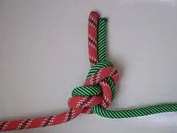
    The offset overhand bend (OOB, ABoK No. 1410) is a knot used to join two ropes together end-to-end. It is formed by holding two rope ends next to each other and tying an overhand knot in them as if they were a single line. Due to its common use in several fields, this bend has become known by many names, such as thumb knot, openhand knot,[1] one-sided overhand knot or flat overhand bend (FOB), though the terms “one-sided” and “flat” are considered incorrect.[2]

    Geometry

    The term ‘offset’ refers to the knot core being displaced from the axis of tension. This geometry allows the knot to more easily translate around an edge – particularly a 90 degree edge.

    Uses

    Long used by weavers to join the ends of yarn, the offset water knot is very old. It was one of the knots likely identified among the possessions of Ötzi the Iceman, who dates from 3300 BC.[3]

    The knot is also tied in a slipped form by mechanical balers to bind straw and hay, but this bend is not practical to use as a binding knot when tied by hand.[1]

    In climbing and mountaineering

    For mountaineers/climbers, there tends to be a strong preference for using knots that are perceived to be relatively easy to tie – even when fatigued or in a less than optimal frame of mind – and so #1410 (Offset overhand bend) is favored. Climbers/canyoners need to retrieve their ropes after an abseil/rappel descent. The ability to retrieve ropes after an abseil descent is crucial – and in many cases, two ropes need to be joined to increase the distance that can be descended in one ‘pitch’. The resulting knot that unites the two ropes needs be secure and stable, have a small footprint, and be resistant to jamming.

    There is controversy over its safety, as it can fail by capsizing under high loads,[4][5][6][7] and some American climbers refer to it as the European death knot, abbreviated to EDK, with some sources recommending against its use.[8][9] Failure of this knot has been implicated in some accidents and near-misses – although post accident retrieval of ropes for examination are usually inconclusive because the ropes have separated (and hence there is no remnant knot to examine).[10][11][12]

    Many sources argue that the name ‘EDK’ is a misnomer, and the knot is safe for abseiling / rappelling, since this does not generate as high forces as a fall. The nominal load during abseiling/rappelling is one person – generally around 1.0kN (approximately 100kg). If the system is configured so the ropes are doubled through the anchor, the joining knot will only be subjected to 50% of the load (ie approximately 0.5kN) – which is well below the instability threshold. With due diligence given to dressing and setting the knot, the risk of capsizing is highly unlikely.[13]

    Several sources recommend adding a second overhand as close as possible to the first (a stacked overhand or double overhand) for most situations, which maintains most of the benefits, while preventing it from capsizing.[9][13][12][11][14][15][16][17] This doubles the overall footprint of the knot, which might increase its likelihood of getting stuck in cracks, but does not harm its ability to pass over edges. There are several different choices of offset knots – all offering varying levels of advantages/disadvantages. Another option is wrapping the strands a second time before passing the tail through (a two-rope version of ABoK #516, also called a double overhand[8] or flat doubled overhand bend[9]) but again, it increases the overall footprint.

    Easily formed in most lines, the offset overhand bend is jam resistant at nominal loads of one person (approximately 100kg). In EN892 climbing ropes, the jamming threshold is thought to be in the vicinity of 3.0kN (300kg). The instability threshold is thought to be above 4.0kN (400kg) – that is, a capsizing event becomes increasingly probable as loads exceed 400kg. It is critically important to pay close attention to dressing and cinching of the knot before attempting to abseil. That is, climbers must exercise due diligence when tying this knot – by pulling firmly on each of the four rope segments – which is necessary to achieve a properly compacted and cinched dressing state.[18]

    Despite questions about this knot’s security, it does present some advantages for use in rappels. Because the knot is offset from the axis of tension, it can translate more easily over uneven surfaces and 90 degree edges than other knots; and it is quickly tied and readily untied. Since a stuck rope on a multi-pitch descent can be catastrophic for climbers, these advantages, along with ease of tying, have led to its popularity. As with all knots used in life critical applications, the tails must be of sufficient minimum length (never less than 200mm in offset knots), and be diligently dressed and fully tightened by pulling individually on all four rope segments.[19]

    Offset overhand bend
    mid rotation state of No. 1410 offset overhand bend

    An interesting yet overlooked fact is that #1410 (offset overhand bend), can be rotated to induce a choking effect to trap and crush the tails. Virtually all testers appear to only examine this knot in its mid-rotation state. It is theorized that this mid-rotation state is in fact the orientation where the structure is most vulnerable to capsizing. In addition, when tying the offset overhand bend using different rope diameters, the thinner diameter rope must be positioned underneath the larger diameter rope. This tactic further inhibits any likelihood of capsizing.

    The offset figure-eight bend, a similar knot using the figure-eight knot, has been used in the belief that its greater size and complexity brings more security. But testing and more than one fatal failure indicate the figure-eight variant to be less secure, more prone to capsize at lower loads, and in capsizing uses more of the ends than does a capsizing overhand bend.[13][19] Moreover, while there is one proper dressing of the overhand bend, there are a couple of dressings for the offset figure eight bend.[2]

    See also

    References

    1. 1 2 Ashley, Clifford W. (1944), The Ashley Book of Knots, New York: Doubleday, p. 45
    2. 1 2 Gommers, Mark (2017-12-24). “Analysis of Offset Overhand Bends”. Professional Association of Climbing Instructors Pty. Ltd (1.6a ed.). Retrieved 2019-02-17. The persistent use of the term ‘flat’ or ‘one-sided’ is incorrect and it is hoped that this paper will assist in correcting the nomenclature.
    3. van der Kleij, Gerre (1996), “On Knots and Swamps”, in Turner, J.C.; van de Griend, P. (eds.), History and Science of Knots, K&E Series on Knots and Everything, vol. 11, Singapore: World Scientific Publishing, pp. 34–35, ISBN 981-02-2469-9
    4. “Flat Overhand Knot Pull Test With Wet Rope”, YouTube (Video), Outdoor Pursuits – Campus Recreation at Auraria, 2014-09-15, archived from the original on 2021-12-12, retrieved 2018-07-10
    5. “Flat Overhand with Backup Knot Dry Pull Test”, YouTube (Video), Outdoor Pursuits – Campus Recreation at Auraria, 2014-11-06, archived from the original on 2021-12-12, retrieved 2018-10-10
    6. “The Breaking Machine”. Vimeo. 0:18 to 0:27. Retrieved 2018-10-10.
    7. Delaney, Richard (2012-04-15), “EDK Edelrid 11mm super static”, YouTube (Video), archived from the original on 2021-12-12, retrieved 2018-10-14
    8. 1 2 Prattley, Grant (June 2016). “Which bends for joining ropes?” (PDF). Over The Edge Rescue. Retrieved 2019-02-17. [2016 version:] The Double Overhand has the best all round performance. … [2015 version:] The overhand is not a recommended bend for tying two ropes for live load due to the low break strength and failure by rolling. … Double overhand is a recommended bend
    9. 1 2 3 Prattley, Grant (2020-10-14). “Which bends for joining ropes? – Update”. Over The Edge Rescue. Retrieved 2020-10-15. Overhand EDK … Not recommended for canyoning. … – Max force is low well below 10kN, the bend rolls off the end, multiple major rolls. … either the Double Overhand or the Stacked Overhand bend are recommended for canyoning
    10. Magnuson, Mark. “Use of the Overhand Knot for Rappels”. Cragmont Climbing Club. Retrieved 2018-07-10.
    11. 1 2 Gaines, Bob; Martin, Jason D. (2014-05-20). Rock Climbing: The AMGA Single Pitch Manual. Rowman & Littlefield. p. 84. ISBN 9781493009626. In one such rappelling accident in recent times (in the Tetons, September 1997), the flat overhand failed when it was sloppily tied with too short of a tail. … For added security it can be easily backed up simply by tying another flat overhand above the first one, although this adds bulk.
    12. 1 2 Kirkpatrick, Andy. “The Ultimate Abseil Knot”. Retrieved 2019-02-17. AND THE BEST JOINING KNOT IS… the double overhand. … During year I used the Simple Overhand Knot to rappel. But one day I almost saw my climbing partner falling because this simple knot.
    13. 1 2 3 Moyer, Tom (1999-11-09), Rope and Gear Testing: Pull Tests of the “Euro Death-Knot”, Adding a safety by tying a second overhand on top of the first is probably a good idea.
    14. Reid, Stephen (2019). “Abseil Knots”. Needle Sports. Retrieved 2026-04-16. As a result of all these findings we are convinced that what we term the Double Overhand is the best knot (if not the safest) to use when joining two ropes together for abseiling.
    15. Jones, Tom (May 8, 2012). “How to Tie Two Ropes Together”. Canyoneering USA. Retrieved 2019-02-17. the preferred knot for connecting rope is the European Death Knot … WITH a back-up knot.
    16. Martin, Jason D. (March 9, 2009). “The Euro Death Knot”. American Alpine Institute. Retrieved 2019-02-17. Most guides tie a backup by adding a second overhand bend next to the first.
    17. Geldard, Jack (2 October 2016). “SKILLS: Abseil Knots Explained”. UKClimbing. Retrieved 2019-02-17. For normal abseiling, if the ropes are dry then I use a well-tied, neat, single overhand knot with ample tails (30cm). If I was double loading the ropes with 2 people at once, or if the ropes were icy, I use a double overhand knot.
    18. Cyrus Lawrence Day (1986), The Art of Knotting and Splicing (4th ed.), Annapolis: Naval Institute Press, pp. 52–53
    19. 1 2 Soles, Clyde (2004), The Outdoor Knot Book, Seattle: The Mountaineers Books, pp. 125–127, ISBN 978-0-89886-962-0

    This article is adapted from “Offset overhand bend” on Wikipedia, written by its contributors, and used under CC BY-SA 4.0. Text on this page is available under the same licence. Source snapshot: Wikipedia via Kiwix, 2026-07-20.
  • Artillery loop

    Artillery loop
    Artillery loop
    Names Artillery loop, Artilleryman’s knot, Manharness knot,[1] Manharness loop, Harness loop,[2] Harness hitch,[2] Belayer’s hitch,[3] Sandy Douglass knot[4]
    Category Loop
    Related Farmer’s loop, Alpine butterfly knot, Span loop, Marlinespike hitch
    Releasing Non-jamming
    Caveat Must have load, may slip unexpectedly under tension creating a running knot or noose
    ABoK #153, #428, #532,[5] #1050, #1051

    The artillery loop[1] is a knot with a loop on the bight for non-critical purposes. The artillery loop must have the loop loaded or it will slip and contract easily. It is an inferior knot to the alpine butterfly knot,[2] possibly dangerously so, in that it can be yanked out of shape and turn into a running knot or noose.[6]

    Budworth states that this knot is often described as being best suited to take a load on only one of the ends, but reliable information on which end is difficult to find.[7]

    Tying the knot

    • Artillery loop step by step
      Artillery loop step by step
    • Finished Artillery loop
      Finished Artillery loop

    Usage

    The name harness loop derives from the fact that the knot was used when assisting horses on difficult terrain.[7] Similarly, the name artillery loop or artilleryman’s hitch derives from the fact that it was used when hauling field artillery into position.[7]

    See also

    Notes and references

    1. 1 2 Ashley, Clifford W. (1944), The Ashley Book of Knots, New York: Doubleday, p. 32
    2. 1 2 3 Ashley, Clifford W. (1944), The Ashley Book of Knots, New York: Doubleday, p. 191
    3. Gregory, John Forrest (1989). Rock sport: tools, training, and techniques for climbers (1st ed.). US: Stackpole books. p. 41. ISBN 0811722961.
    4. “The Sandy Douglass Knot”. Knotting Matters. No. 77. International Guild of Knot Tyers. p. 34-35. ISSN 0959-2881.
    5. Entry #532 on page 87 of The Ashley Book of Knots shows a diagram of the alpine butterfly knot under the name harness loop. Ashley appears to have illustrated or named the incorrect knot in this case. The butterfly knot, under the name Lineman’s Loop, is shown and discussed as a distinct and specific knot throughout the rest of the book.
    6. Cyrus Lawrence Day (1986), The Art of Knotting and Splicing (4th ed.), Annapolis: Naval Institute Press, pp. 80–81
    7. 1 2 3 Budworth, Geoffrey (2012). The Knot Book. London: Constable & Robinson. p. 106. ISBN 978-0716023043.

    External links


    This article is adapted from “Artillery loop” on Wikipedia, written by its contributors, and used under CC BY-SA 4.0. Text on this page is available under the same licence. Source snapshot: Wikipedia via Kiwix, 2026-07-20.
  • Offset figure-eight bend

    Offset figure-eight bend
    Offset figure-eight bend
    Names Offset figure-eight bend,
    flat figure-eight bend[1],
    abnormal figure-eight bend[2]

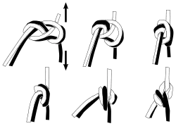
    The offset figure-eight bend is a poor knot that has been implicated in the deaths of several rock climbers.[1][3][4][5][6] The knot may capsize (invert) under load, as shown in the figure, and this can happen repeatedly.[7] Each inversion reduces the lengths of the tails. Once the tails are used up completely, the knot comes undone.

    Offset figure-eight bend
    An offset figure-eight knot inverting itself

    More secure knots for this purpose are the Flemish bend (the “figure eight bend”), (doubled) offset overhand bend, or double fisherman’s knot.

    See also

    References

    1. 1 2 Moyer, Tom (1999-11-09). “Pull Tests of the “Euro Death-Knot”. Rope and Gear Testing. Retrieved 2018-07-10.
    2. “Rock Climbing Tech Tips: Joining Two Ropes”. Chockstone.org. Retrieved 2018-07-10.
    3. “Report from Zion Rap Accident Survivor”. groups.google.com. Retrieved 2026-04-09. grab both ropes together and then tie a regular single fig-eight knot in both ropes at once. … single fig-eight in one rope then follow this through with the other rope – we did NOT do this
    4. Jackson, Jeff. “Rappel Knot Fails, Climber Falls to Death on the Goat Wall”. Rock and Ice. Archived from the original on 2016-12-05. Retrieved 2018-07-10. Erps had rigged the previous rappels using a flat figure 8
    5. “Rappel Failure – Inadequate Knot”. Rock and Ice Magazine. Retrieved 2026-04-09. it’s likely he too used a at figure-8; it’s unknown if he backed up the knot. Testing has shown the at figure-8 is prone to rolling or “capsizing” under loads
    6. “Fall on Rock, Failure of Rappel-Knot Came Undone, No Hard Hat, West Virginia, Seneca Rocks”. Accidents in North American Mountaineering. The American Alpine Club. 1995.
    7. Dahlberg, Robin. “Cross load test of common climbing knots”. Vimeo. 0:08-0:35. Retrieved 2020-06-10.

    This article is adapted from “Offset figure-eight bend” on Wikipedia, written by its contributors, and used under CC BY-SA 4.0. Text on this page is available under the same licence. Source snapshot: Wikipedia via Kiwix, 2026-07-20.
  • Nubian wig

    Nubian wig
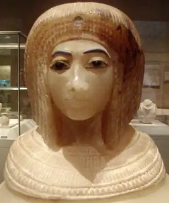
    Canopic Jar (07.226.1) with a Lid in the Shape of a Royal Woman’s Head (30.8.54); ca.1349–1336 B.C. or shortly thereafter; Travertine (Egyptian alabaster), blue glass, obsidian, unidentified stone; Lid (30.8.54): H. 18.2 cm (7 3/16 in); diam. 16.6 cm (6 9/16 in); The Metropolitan Museum of Art
    Nubian wig
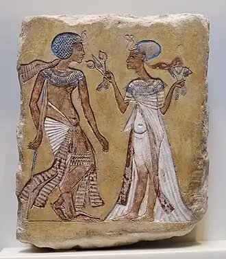
    Artist’s sketch: Walk in the Garden; limestone; New Kingdom, 18th dynasty, c. 1335 BC. Egyptian Museum Berlin, Inv. no. 15000 (donated by James Simon in 1920).

    In Ancient Egyptian society, hair was an embodiment of identity.  It could carry religious and erotic significance and portray information about gender, age, and social status.[1] During the New Kingdom, more elaborate hairstyles for men and women, incorporating curls and plaits, began to be favored over the traditional, simple hairstyles of the Old and Middle Kingdoms.[2]

    Nubian wigs, which Ancient Egyptians grew fond of during the Amarna period, were meant to mimic the short curly hair that Nubian tribespeople wore.[3][4] Egyptologists believe that the Nubian wig was adopted by Queen Nefertiti after witnessing the hairstyle being worn by Nubians in the Pharaoh’s army.[5] Though there has been a discussion on what qualifies as a Nubian wig, some arguing layered wigs known as “duplex” styles that include curls and plaits may also be Nubian wigs. Still, many refer to this as a Nubian style and not a Nubian wig.[4]

    In general, wigs in Ancient Egypt were almost entirely confined to the elite due to their price. Even when wigs were made of inexpensive materials like plant fibers, the sophisticated craftsmanship required to make wigs proved costly.[2][6]

    Iconography

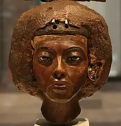
    One can see Nubian wigs in the form of reliefs, statues, and paintings. They are a prime factor in determining the gender of figures in Ancient Egyptian art, as royal women exclusively wear them.[7]  It is characterized by its short bushy appearance with rows of curls that frame the brow and sides of the face.  The feature that requires the most attention is located on the neck.[7] In Nubian wigs, the hair is cut to expose the nape of the neck, which distinguishes it from a similar headdress where the nape of the neck is not exposed, and the hair falls towards the shoulders.  Royal men exclusively wear this alternative style and can be seen in the left image titled Walk in the Garden.[7]

    Techniques and composition

    Wigs were composed of various materials such as human hair, wool, plant fibers, and horsehair.[2]  The most expensive wigs were made of human hair or black sheep wool, or both.[2] In addition to the hair, false or human, Ancient Egyptians used beeswax and resin to hold the style in place on a mesh cap.[8]

    One wig specifically, titled wig by The British Museum, has been studied extensively. Efforts to study other wigs are scarce due to the fragile nature or incompleteness of the wigs after thousands of years. Though this wig is the “duplex” style that men wore and is referenced above, its condition gives historians insight into how Ancient Egyptians created wigs.[8]

    To begin the process of making a wig, a wigmaker must have first collected hair.  After a wigmaker collected enough hair, the hair was washed and separated into individual locks with about 400 strands per lock.[6] Construction could then begin on a wooden wig mount very similar to what modern wigmakers would use.  The wig achieved the mesh base by laying hair down vertically and horizontally across each other.  The base layer was kept in place by knotting and folding the hair back over itself and then was further reinforced by a mixture of two-thirds beeswax and one-third conifer resin.[6] To hook curls to the mesh layer, the curl was looped around the mesh and then fastened by fifteen individual hairs, called a “sub-strand” that was tired around the stem of the curl.  Wigs could take up to 200 hours to complete and could take even longer if plaits were styled on the wooden wig mount, as they probably were in ancient times.[6]

    Gallery

    • Bust of Tiye, now in the Ägyptisches Museum in Berlin, Germany
      Bust of Tiye, now in the Ägyptisches Museum in Berlin, Germany
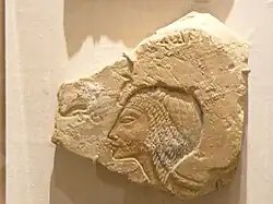
    • Relief depicting the queen, Nefertiti (E.GA.4530.1943); ca.1352-1336 B.C.; Limestone, Painted; The Fitzwilliam Museum Cambridge
      Relief depicting the queen, Nefertiti (E.GA.4530.1943); ca.1352-1336 B.C.; Limestone, Painted; The Fitzwilliam Museum Cambridge
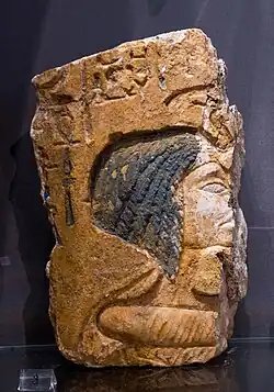
    • Late Image of Nefertiti (35.1999); Sandstone, pigment; ca.1352-1336 B.C.; 11 9/16 x 3 15/16 x 17 1/8 in. (29.3 x 10 x 43.5 cm); Brooklyn Museum, Gift of the Egypt Exploration Society
      Late Image of Nefertiti (35.1999); Sandstone, pigment; ca.1352-1336 B.C.; 11 9/16 x 3 15/16 x 17 1/8 in. (29.3 x 10 x 43.5 cm); Brooklyn Museum, Gift of the Egypt Exploration Society
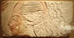
    • Relief Depicting the Purification of Queen Kiya (?) (1985.328.8); Limestone, paint; ca. 1353–1336 B.C.; H. 22.8 × l. 47 × d. 2.5 cm (9 × 18 1/2 × 1 in.); Metropolitan Museum
      Relief Depicting the Purification of Queen Kiya (?) (1985.328.8); Limestone, paint; ca. 1353–1336 B.C.; H. 22.8 × l. 47 × d. 2.5 cm (9 × 18 1/2 × 1 in.); Metropolitan Museum

    References

    1. Robins, Gay (1999). “Hair and the Construction of Identity in Ancient Egypt, c. 1480-1350 B.C.”. Journal of the American Research Center in Egypt. 36: 55–69. doi:10.2307/40000202. ISSN 0065-9991. JSTOR 40000202.
    2. 1 2 3 4 Sherrow, Victoria (31 March 2021). Encyclopedia of hair : a cultural history. Bloomsbury Academic. ISBN 978-1-4408-7348-5. OCLC 1242794418.
    3. Watterson, Barbara (2013). Women in ancient Egypt. Amberley. ISBN 978-1-4456-1020-7. OCLC 857656435.
    4. 1 2 Samson, Julia (August 1973). “Amarna Crowns and Wigs: Unpublished Pieces from Statues and Inlays in the Petrie Collection at University College, London”. The Journal of Egyptian Archaeology. 59: 47–59. doi:10.2307/3856096. ISSN 0307-5133. JSTOR 3856096.
    5. “Brooklyn Museum”. www.brooklynmuseum.org. Retrieved 2021-05-07.
    6. 1 2 3 4 Fletcher, Joann; Salamone, Filippo (2016). “An Ancient Egyptian Wig: Construction and Reconstruction”. Internet Archaeology (42). doi:10.11141/ia.42.6.3. ISSN 1363-5387.
    7. 1 2 3 Aldred, Cyril (February 1957). “Hair Styles and History”. The Metropolitan Museum of Art Bulletin. 15 (6): 141–147. doi:10.2307/3257776. ISSN 0026-1521. JSTOR 3257776.
    8. 1 2 Cox, J. Stevens (1977). “The Construction of an Ancient Egyptian Wig (c. 1400 B.C.) in the British Museum”. The Journal of Egyptian Archaeology. 63: 67–70. doi:10.2307/3856302. ISSN 0307-5133. JSTOR 3856302.

    This article is adapted from “Nubian wig” on Wikipedia, written by its contributors, and used under CC BY-SA 4.0. Text on this page is available under the same licence. Source snapshot: Wikipedia via Kiwix, 2026-07-20.
  • Arnold invariants

    Arnold invariants
    Mathematician Vladimir Arnold

    In mathematics, particularly in topology and knot theory, Arnold invariants are invariants introduced by Vladimir Arnold in 1994[1] for studying the topology and geometry of plane curves. The three main invariants— J + {\displaystyle J^{+}} {\displaystyle J^{+}}, J {\displaystyle J^{-}} {\displaystyle J^{-}}, and S t {\displaystyle St} {\displaystyle St}—provide ways to classify and understand how curves can be deformed while preserving certain properties.[2]

    Background

    The fundamental context for Arnold invariants comes from the Whitney–Graustein theorem, which states that any two immersed loops (smooth curves in the plane) with the same rotation number can be deformed into each other through a series of continuous transformations.[3] These transformations can be broken down into three elementary types: direct self-tangency moves (where two portions of the curve become tangent with aligned directions, either creating or eliminating two self-intersection points), inverse self-tangency moves (similar to direct moves, but the tangent directions are opposite), and triple point moves (where three portions of the curve intersect at a single point).[4]

    J± invariants

    The J + {\displaystyle J^{+}} {\displaystyle J^{+}} and J {\displaystyle J^{-}} {\displaystyle J^{-}} invariants keep track of how curves change under these transformations and deformations. The J + {\displaystyle J^{+}} {\displaystyle J^{+}} invariant increases by 2 when a direct self-tangency move creates new self-intersection points (and decreases by 2 when such points are eliminated), while J {\displaystyle J^{-}} {\displaystyle J^{-}} decreases by 2 when an inverse self-tangency move creates new intersections (and increases by 2 when they are eliminated). Neither invariant changes under triple point moves. A fundamental relationship between these invariants is that their difference equals the total number of self-intersection points in the curve. That is,

    J + ( c ) J ( c ) = number of self-intersection points of  c {\displaystyle J^{+}(c)-J^{-}(c)={\text{number of self-intersection points of }}c} {\displaystyle J^{+}(c)-J^{-}(c)={\text{number of self-intersection points of }}c}.[5]

    Mathematicians Oleg Viro and Eugene Gutkin discovered an explicit formula for calculating J {\displaystyle J^{-}} {\displaystyle J^{-}}:

    J ( c ) = 1 R wind ( c , R ) 2 + q meanwind ( c , q ) 2 {\displaystyle J^{-}(c)=1-\sum _{R}{\text{wind}}(c,R)^{2}+\sum _{q}{\text{meanwind}}(c,q)^{2}} {\displaystyle J^{-}(c)=1-\sum _{R}{\text{wind}}(c,R)^{2}+\sum _{q}{\text{meanwind}}(c,q)^{2}}[5]

    where R {\displaystyle R} {\displaystyle R} ranges over the regions into which c {\displaystyle c} {\displaystyle c} divides the plane, wind ( c , R ) {\displaystyle {\text{wind}}(c,R)} {\displaystyle {\text{wind}}(c,R)} is the winding number around a point in region R {\displaystyle R} {\displaystyle R}, and meanwind ( c , q ) {\displaystyle {\text{meanwind}}(c,q)} {\displaystyle {\text{meanwind}}(c,q)} is the mean winding number at each self-intersection point q {\displaystyle q} {\displaystyle q}. For example, a curve with k {\displaystyle k} {\displaystyle k} curls in standard form has J + = 2 k {\displaystyle J^{+}=-2k} {\displaystyle J^{+}=-2k} and J = 3 k {\displaystyle J^{-}=-3k} {\displaystyle J^{-}=-3k}, while a simple circle has J + = J = 0 {\displaystyle J^{+}=J^{-}=0} {\displaystyle J^{+}=J^{-}=0}.[4]

    Bridges and channels

    In 2002, mathematicians Catarina Mendes de Jesus and Maria Carmen Romero Fuster introduced the concepts of bridges and channels for plane curves to facilitate the calculation of Arnold invariants.[6] A bridge consists of introducing a rectangle in the complement of the curve in the plane while respecting orientations, decomposing a given curve into two smaller curves with known invariants. The invariant of the original curve can then be obtained as a function of the invariants of these two component curves and the index of the bridge relative to the original curve. This decomposition technique is particularly powerful for analyzing curves with double points.

    An important theorem regarding this decomposition states that a curve with n {\displaystyle n} {\displaystyle n} double points is a tree-like curve if and only if it admits a decomposition into exactly n curves of types K 0 {\displaystyle K_{0}} {\displaystyle K_{0}} and K 2 {\displaystyle K_{2}} {\displaystyle K_{2}} with bridges having no double points, or a decomposition into exactly n + 1 {\displaystyle n+1} {\displaystyle n+1} curves of type K 1 {\displaystyle K_{1}} {\displaystyle K_{1}} (isotopic to the circle) with bridges having double points.[7] This result proved a conjecture originally proposed by Arnold regarding the formulas for families of tree-like curves. The bridge and channel technique provides a systematic method for computing Arnold invariants for plane curves in terms of simpler curves with at most one double point.

    See also

    • Plane curve
    • Knot invariant
    • Whitney–Graustein theorem
    • Differential topology

    References

    1. Arnold, V. I. (1994). Topological Invariants of Plane Curves and Caustics. University Lecture Series, Vol. 5, American Mathematical Society.
    2. Mai, Alexander (2022). “Introduction to Arnold’s J+-Invariant”. arXiv:2210.00871.
    3. Whitney, H. (1937). “On regular closed curves in the plane”. Compositio Mathematica, 4, 276-284.
    4. 1 2 Moraes, Simone (2018). “Invariants of Closed Plane Curves”. Federal University of Bahia.
    5. 1 2 Professor Paul Seidel online lecture notes at https://ocw.mit.edu/courses/18-900-geometry-and-topology-in-the-plane-spring-2023/mit18_900s23_lec17.pdf
    6. Mendes de Jesus, C.; Romero Fuster, M. C. (2002). “Bridges, channels and Arnold’s invariants for generic plane curves”. Topology and its Applications, 125, 505-524.
    7. Aicardi, F. (1994). “Tree-like Curves”. In: Singularities and Bifurcations. Advances in Soviet Mathematics, 21, AMS, Providence, 1-36.

    Further reading

    • Santa Rosa, Lílian Neves (2010). Arnold Invariants of Plane Curves. Master’s Thesis, Federal University of Viçosa.
    • Mendes de Jesus, C. Topological Invariants of Generic Maps from Oriented Compact Surfaces to the Plane. Doctoral Thesis, PUC-RIO, 2001.
    • Moraes, Simone M.; Sánchez, Catarina M. J. “Invariants of Closed Plane Curves”. Proceeding Series of the Brazilian Society of Applied and Computational Mathematics, Vol. 3, N. 1, 2015.
    • Lagemann, Anna Marie; von der Mosel, Heiko (Thesis advisor); Hryniewicz, Umberto (Thesis advisor); Reiter, Philipp (Thesis advisor). Variational approach to study Arnold’s invariants of immersed planar curves RWTH Aachen University (2023) PhD Thesis

    Original source


    This article is adapted from “Arnold invariants” on Wikipedia, written by its contributors, and used under CC BY-SA 4.0. Text on this page is available under the same licence. Source snapshot: Wikipedia via Kiwix, 2026-07-20.

  • Noose

    Noose
    Noose

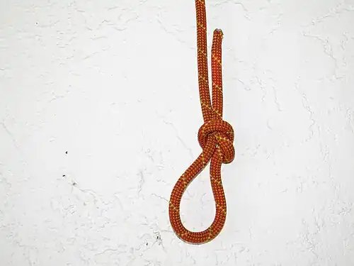
    A noose knot tied in kernmantle rope
    Names Noose, running knot
    Category Loop
    Related Slip knot, overhand knot, double overhand noose, hangman’s knot, running bowline, arbor knot
    Releasing Non-jamming
    Typical use Animal snares, knitting, hanging device, self tightening end loop
    ABoK #8, #43, #1114,[1] #1789, #1803, #1825
    Instructions

    A noose is a loop at the end of a rope in which the knot tightens under load and can be loosened without untying the knot. The knot can be used to secure a rope to a post, pole, or animal but only where the end is in a position that the loop can be passed over.

    Tying

    Noose
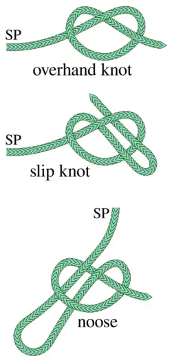
    The noose knot is a slipped version of the overhand knot

    The knot is tied by forming a turn in the end of a rope, and then passing a bight in the standing part through. The noose knot is a slipped version of the overhand knot.

    Use in hanging

    The knot most closely associated with execution is the hangman’s knot, which is also known as the “hangman’s noose”. Tying is similar to the original noose, but many turns are wrapped around the loop. The reason for this was to make the hanging more humane, as it would break the person’s neck, killing the person instantly, rather than strangling them to death. A similar method is also commonly used for suicide.

    Use in intimidation and hate-based racial politics

    In the United States, a noose is sometimes left as a message in order to intimidate people, as it was the main object used in segregation era lynchings.[2][3] In 2022, a bill to make lynching a federal hate crime was passed.[4] It is illegal to display a noose in a threatening manner in Virginia,[5] New York and Connecticut.[6]

    Austin Reed Edenfield, a former student of the University of Mississippi, pled guilty in 2016 to a federal civil-rights crime, acknowledging that he and Graeme Phillip Harris had tied a noose and a flag of Georgia around the neck of a statue honoring James Meredith, the university’s first African-American student.[7] Harris was sentenced to prison and Edenfield to probation and community service.[8]

    In September 2019, Andrew M. Smith, a University of Illinois student, was arrested for placing a noose in a campus elevator. “The incident [came] just months after black employees filed a class-action lawsuit against the campus, alleging they faced racial harassment and were exposed to threats of racial violence, such as nooses, swastikas, KKK garb, racist graffiti, and confederate flags.”[9] He was sentenced to supervision, public service, and a $75 fine.[10]

    In November 2022, a noose was found on an Obama Presidential Center construction site.[11]

    In July 2025, a noose was found during construction at the New Nissan Stadium.[12]

    Bubba Wallace incident

    In July 2020 a garage assigned to African-American NASCAR driver Bubba Wallace had been found to contain a “garage door pull rope fashioned like a noose”. After the discovery, which was made by a crew member for Richard Petty Motorsports at the Alabama racetrack, NASCAR was alerted and contacted the FBI, which sent 15 agents to the track to investigate. After the FBI investigation the authorities said the rope had been hanging there since last fall and thus was not a hate crime targeting Wallace. The agencies said no crime was committed and the evidence did not support federal charges.[13][14] The actions of NASCAR, especially NASCAR president Steve Phelps’s claim of it being a hate crime without investigation have been criticized.[15] Holman W. Jenkins Jr. on The Wall Street Journal claimed the controversy and media furor concerning the incident could have been prevented by not contacting the FBI and NASCAR authorities quickly checking the video surveillance by themselves, since NASCAR already tightly controls and surveils access to its garages.[16]

    See also

    Further reading

    • Jack Shuler, The Thirteenth Turn: A History of the Noose, Public Affairs, 2014, ISBN 9781610391368

    References

    1. Ashley, Clifford W. (1993) [1944], The Ashley Book of Knots, New York: Doubleday, p. 204, ISBN 0-385-04025-3
    2. Noose incidents evoke segregation-era fears, NBC News. October 10, 2007.
    3. Coast Guard tries to deal with noose incidents, CNN. October 4, 2007.
    4. McDaniel, Eric; Moore, Elena (2022-03-29). “Lynching is now a federal hate crime after a century of blocked efforts”. NPR. Retrieved 2022-03-29.
    5. Displaying noose on property of another or a highway or other public place with intent to intimidate; penalty, Code of Virginia. October 27, 2017.
    6. Noose displays provoke new state penalties Archived 2012-04-12 at the Wayback Machine, Stateline.org. June 6, 2008.
    7. Svrluga, Susan (March 24, 2016). “Former Ole Miss student pleads guilty to hanging noose around statue honoring the first black student”. Washington Post.
    8. “2nd ex-Ole Miss student sentenced in statue vandalism”. The Clarion-Ledger. Associated Press. Retrieved 2021-05-02.
    9. Melendez, Pilar (September 3, 2019). “University of Illinois Student Charged With Hate Crime After Noose Found Hanging in Dorm Elevator: Officials”. Daily Beast.
    10. Staff, WICS/WRSP (2020-05-12). “Former U of I student pleads guilty in noose incident”. WRSP. Retrieved 2021-05-02.
    11. “Work halted at Obama Presidential Center after noose is found”. Chicago Tribune. 10 November 2022. Retrieved 2022-11-11.
    12. “Police: Noose found at Titans’ new stadium site; work halted”. ESPN. 18 July 2025. Retrieved 2025-07-18.
    13. ‘The noose was real’: Nascar releases photo from Bubba Wallace’s garage”. the Guardian. Associated Press. 2020-06-25. Retrieved 2021-08-12.
    14. “FBI determines Wallace not victim of hate crime”. ESPN.com. 2020-06-23. Retrieved 2021-08-12.
    15. “NASCAR’s regret over the Bubba Wallace noose situation”. Beyond the Flag. 2021-01-01. Retrieved 2021-08-12.
    16. Jenkins, Holman W. Jr. (2020-06-26). “Opinion | Bubba Wallace and the ‘Noose’ That Wasn’t”. Wall Street Journal. ISSN 0099-9660. Retrieved 2021-08-12.

    This article is adapted from “Noose” on Wikipedia, written by its contributors, and used under CC BY-SA 4.0. Text on this page is available under the same licence. Source snapshot: Wikipedia via Kiwix, 2026-07-20.